DELTALab — User Guide
Who this is for: geochemists processing clumped and bulk stable-isotope data (δ¹³C, δ¹⁸O, Δ₄₇, Δ₄₈).
App version: 1.0.3 · Guide updated: 2026-11-13
DELTALab turns raw mass-spectrometer output into standardised Δ values and temperatures. It corrects the background, puts your data on a reference frame and converts Δ to temperature. You get replicate and sample tables, diagnostic plots and exports you can use in a paper. The clumped-isotope maths gives the same numbers as D47crunch (Daëron 2021) and D47calib (Daëron & Vermeesch 2024).
New to DELTALab? Read chapter 1 (the seven key words). Come back to the other chapters when you need them.
How this guide is written:
- Button and menu names are in bold, exactly as they appear in the app.
- "→" means "then click". For example, Contacts → Learning Routine.
- Every chapter stands on its own, so you can open any one of them directly.
1. Key words
DELTALab uses seven words everywhere.
Acquisition — One block of measurement cycles from the instrument. Each cycle records the sample and reference-gas beams at m/z 44–49 (plus the 47.5 half-mass, if your instrument has that cup). An acquisition is the smallest unit you import.
Replicate — One analysis of one sample. DELTALab joins back-to-back acquisitions of the same sample into one replicate. Standardisation, exclusion and temperature all work on replicates.
Sample — The material you analysed, known to DELTALab by its sample name. Replicates with exactly the same sample name are one sample, also when they are in different sessions. A sample is either a standard or an unknown, a sample you want a result for. In the app, Samples on its own (the summary bar, Filter to) means the unknowns only.
Session — A batch of replicates that you process together, usually one instrument run. A session has its own background correction, standardisation fit, reference gas, acid reaction temperature and mass spectrometer. Almost every screen works on a session or a group of sessions.
Standard (also: reference material) — A sample with an accepted value, such as ETH-1 to ETH-4, IAEA-C1/C2, equilibrated gases or an in-house carbonate. Their values live in Settings → Reference material (chapter 7). A standard you use to constrain a fit is simply called a standard here.
Standardisation — Moving your raw Δ values (Δ₄₇ raw) onto a community reference frame (Δ₄₇, for example I-CDES). DELTALab does this by fitting a transfer function through your standards. The fit can also follow a slow drift over time. Bulk Standardization does the same for δ¹³C and δ¹⁸O.
Isotope system — What you are measuring: Clumped Isotopes (Δ₄₇) or Dual Clumped (Δ₄₇ and Δ₄₈). You choose it in the menu of the top bar (chapter 2). It decides which tabs you see and which Δ you process.
Raw values are kept apart from results
The voltages of every cycle are stored at import and never changed. DELTALab
calculates the raw values (δ¹³C, δ¹⁸O, Δ₄₇ raw, Δ₄₈ raw) from them.
Standardisation, temperature conversion and the δ¹⁸O acid correction never overwrite a raw value. Each writes to its own columns, so you can run them again as often as you like without losing data.
A raw value changes only when DELTALab calculates it again from the cycles:
- after a Negative Background Correction (chapter 5);
- when you exclude cycles or an acquisition (chapter 4.1);
- when you change a session's reference gas (chapter 6).
Moving, renaming or deleting replicates does not change the raw value of any other replicate.
Δ₄₇ raw and the standardised Δ₄₇ are separate columns. δ¹³C and δ¹⁸O have one
column each in the Replicate list: it shows the standardised value once Bulk Standardization
has run, and "—" until then. Choose raw in the column's header menu to see the raw value, or
hover over a standardised δ¹³C or δ¹⁸O to see the raw value behind it.
2. Finding your way around
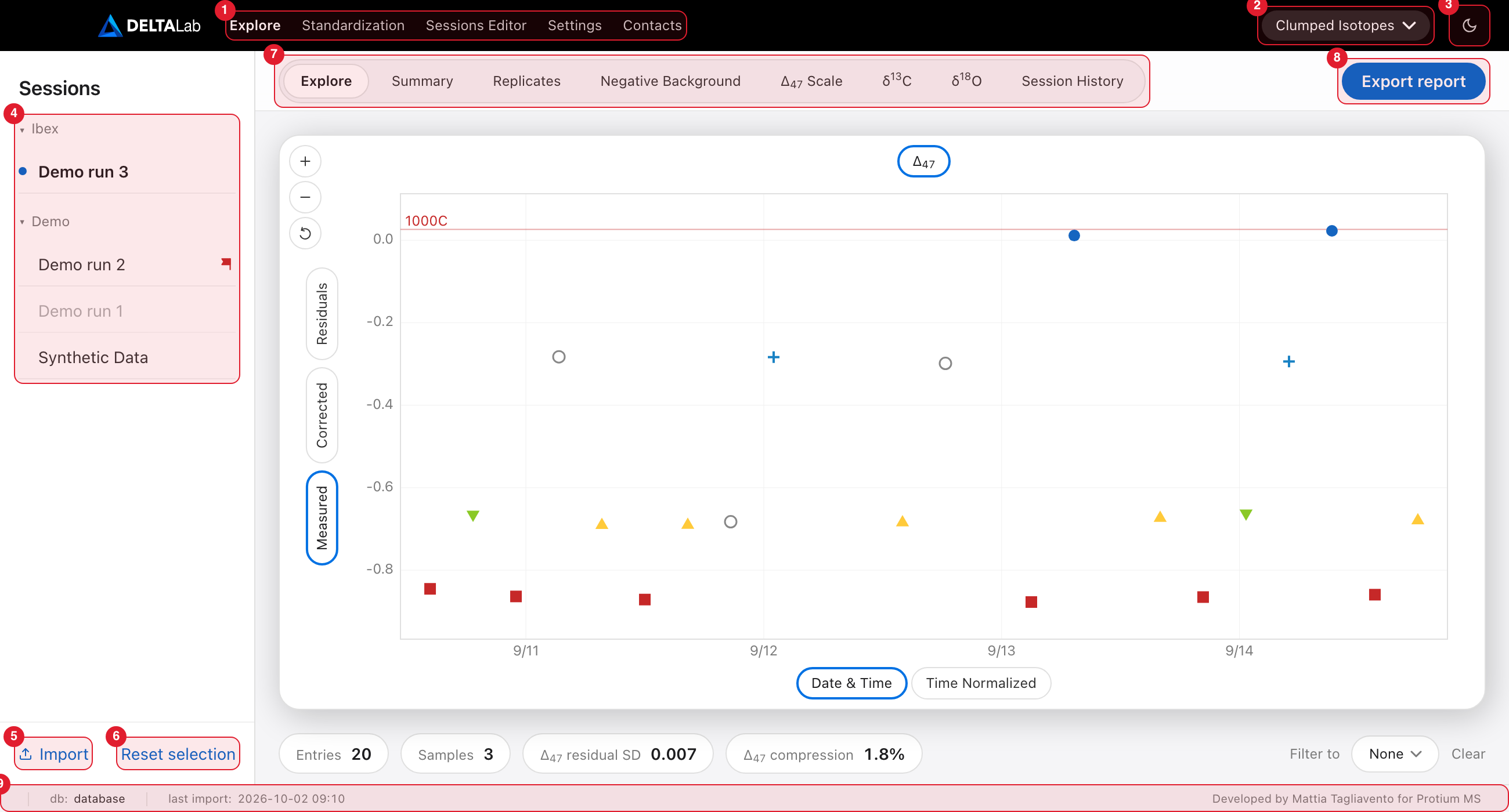
Marked in red: 1 the five pages, 2 the isotope-system menu, 3 the light/dark button, 4 the session list, 5 Import, 6 Reset selection, 7 the tabs of the Explore page, 8 Export report, 9 the status bar.
The top bar
The five pages (1 in the picture). The page you are on is shown in bold.
| Page | What you do there | Chapter |
|---|---|---|
| Explore | Look at your data: plots, tables, exports | 4 |
| Standardization | Process your data | 5 |
| Sessions Editor | Rename, move, split and delete; manage scans | 6 |
| Settings | Standards, instruments, calibrations, databases, backups | 7 |
| Contacts | Version, this guide, the guided tour, feedback | below |
The isotope-system menu (2) chooses Clumped Isotopes or Dual Clumped.
- The menu is shown on the Explore, Standardization, Sessions Editor and Settings pages. Contacts does not need it.
- On Explore it decides which tabs you see.
- On Standardization it decides what you process: Δ₄₇ only, or Δ₄₇ and Δ₄₈.
- On Sessions Editor only the Split session window uses it.
- Your choice stays while you move between pages.
- Every time DELTALab starts, the menu is set to the Default environment you chose in Settings (chapter 7).
The light/dark button (3) switches between light and dark mode. It shows a moon in light mode and a sun in dark mode. DELTALab remembers your choice.
On a Mac the top bar is also the window's title bar: drag an empty part of it to move the window.
The session list (left side)
The Explore, Standardization and Sessions Editor pages have a session list (4). Settings and Contacts do not.
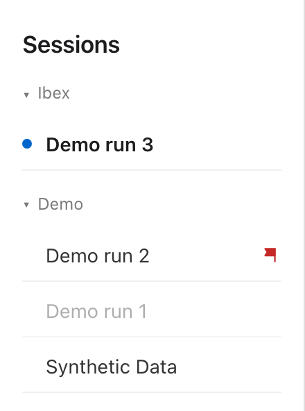
- Sessions are listed newest first (by their most recent replicate).
- If your sessions come from more than one mass spectrometer, they are grouped by instrument. Click a group's name to fold or unfold it. Sessions with no instrument are under Unassigned.
- A selected session is in bold and has a blue dot.
- A session in pale grey is deactivated (chapter 6). You can still open it on Explore and in the Sessions Editor. It is left out of the Standardization page, Export report and the Import window.
- On Explore and Standardization, click a session to select it (any other session is deselected). To select several, hold Cmd (Mac) or Ctrl (Windows) and click each one; Cmd/Ctrl + click a selected session removes it. Reset selection (6) deselects everything.
- On the Sessions Editor one session is always open. Click another one to switch to it.
- Import (5), at the bottom of the list on all three pages, opens the import window (chapter 3). A newly imported session appears in the list straight away.
Important:the tables and plots show every selected session together. Select two runs and the Replicates, Summary and plots show both, merged. This is how you view or standardise several sessions at once.
Each page has its own selection:
- Explore keeps its selection while you visit other pages.
- Standardization starts with nothing selected every time you open it.
- Sessions Editor opens on the newest session every time you open it.
- After a standardisation, Go to Explore and Go to History open the Explore page with the sessions you just processed selected (chapter 5).
The red flag: "standardisation is out of date"
A red flag at the right end of a session's row means its standardisation is out of date. In the picture above, "Demo run 2" has one. Something changed after the last standardisation, for example:
- you excluded or included a replicate;
- you imported more data into the session;
- you moved, renamed or deleted replicates in the Sessions Editor (chapter 6).
The old values stay on screen until you re-run standardisation (chapter 5). Then the flag disappears.
The flag also disappears if you simply undo the change, for example by including again exactly the replicates you had excluded.
A new reference gas or a split works differently: it clears the session's standardised values, so there is no flag. Δ₄₇ shows "—" until you standardise again.
A session with no flag is either up to date or not standardised yet.
The status bar
The thin bar along the bottom of the window (9) is on every page.
- db: the name of the database DELTALab is working on. Hover over it to see the full path of the file. Chapter 7 explains how to change or rename the database, and chapter 8 says where the files are.
- last import: the date and time of your last import.
- On the right is the developer's name.
The Contacts page
The card at the top shows the version of DELTALab you are running, and the developer's name and email address. Below it are two cards.
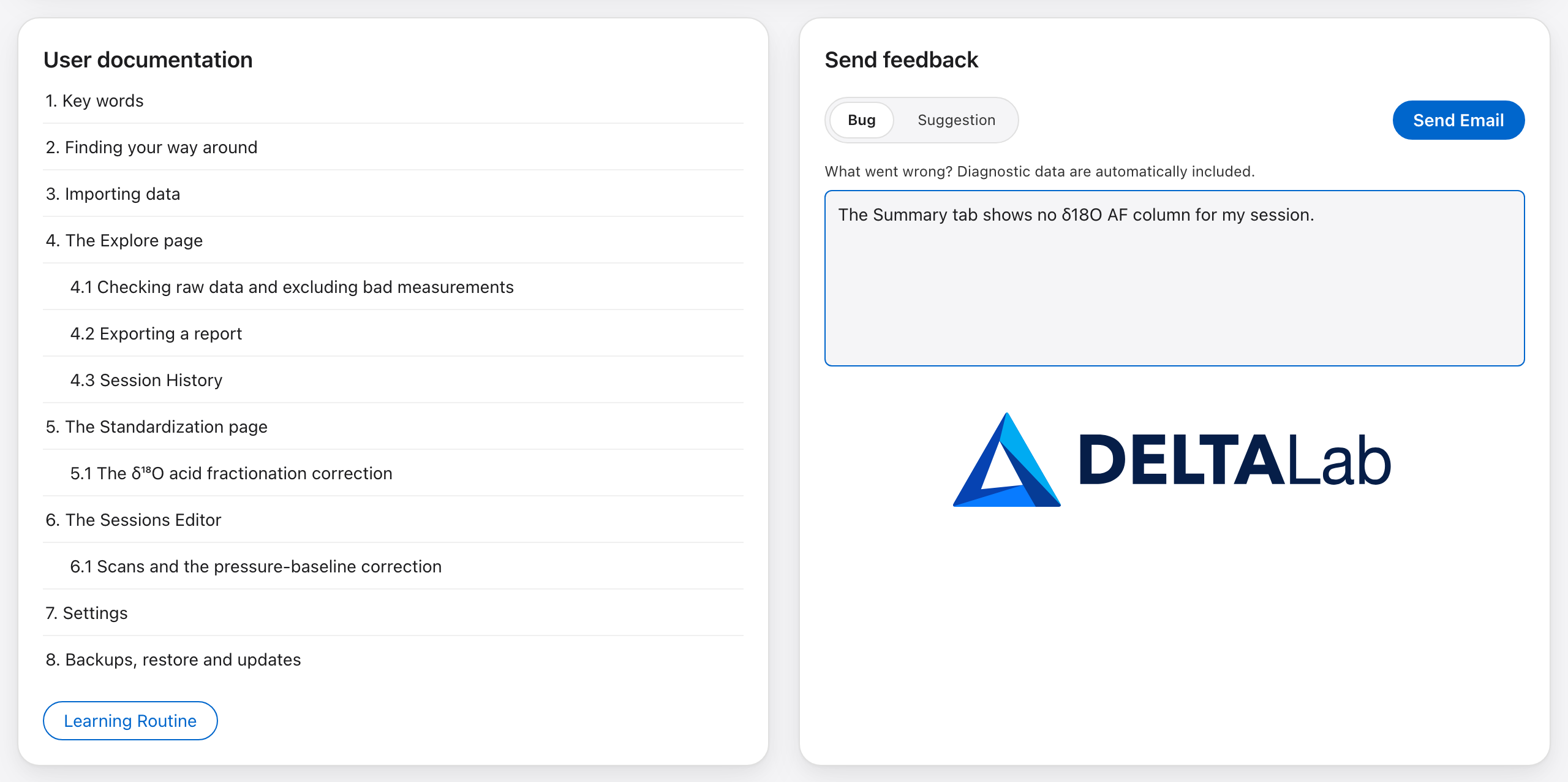
User documentation is this guide.
- Click a chapter to open it in a window.
- A blue link inside a chapter opens the chapter it points to.
- Close the window with ✕, or click outside it.
Learning Routine, under the list of chapters, starts a guided tour of the app.
Send feedback writes an email to the developer for you.
- Choose Bug or Suggestion.
- Type your message in the box.
- Click Send Email. It stays greyed out until you have typed something.
- Your email program opens with the message ready. Nothing is sent until you send it there.
A Bug message also carries a short technical summary: the DELTALab version, your operating system, the name of the database file and the number of rows in each table. It holds no measurement values and no sample names.
3. Importing data
On the Explore page, click Import at the bottom of the session list (chapter 2). The import window has four tabs, one for each kind of file:
| Tab | What you import |
|---|---|
| Qtegra | CSV files exported from Qtegra |
| Isodat | .did files, read directly |
| Wintel | Not built yet. The tab only says "Coming soon...". |
| Easotope | A whole Easotope database |
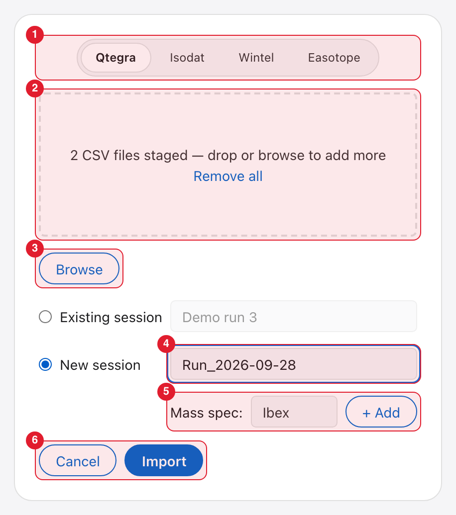
Marked in red: 1 the tabs, 2 the drop area, 3 Browse, 4 the session, 5 the mass spectrometer, 6 Cancel and Import.
The steps for Qtegra and Isodat files
- Choose the tab (1).
- Drop your files on the drop area (2), or click Browse (3). The drop area then says how many files are waiting.
- Choose the session the data goes into (4).
- For a new session, choose its mass spectrometer (5).
- Click Import (6). It stays greyed out until at least one file is waiting.
When the import is done the session is in the session list. If everything in your files was imported, the window closes. If something was left out, the window stays open and tells you what and why (see "When DELTALab leaves something out" below).
Good to know:
- You can add files in several goes. Dropping or browsing again adds to the files that are waiting. A file that is already waiting is not added twice.
- Remove all, in the drop area, forgets the waiting files so you can start again.
- CSV files and
.didfiles cannot wait together. If CSV files are waiting and you choose.didfiles (or the other way round), the new files replace the old ones. - If something is missing when you click Import, there is no message. The field you still have to fill, the session name or the mass spectrometer, gets a red outline.
- Cancel, or a click outside the window, closes it and forgets the waiting files.
Qtegra (CSV files)
Choose one or more Qtegra CSV exports. Several files are fine: they are all added to the same session.
- DELTALab detects whether the file uses commas or semicolons.
- DELTALab works out whether the dates are written day-first or month-first. It decides once for all the files you import together, and then checks every row.
- If the dates of a file could be read either way, that file is refused rather than
risk putting your replicates in the wrong order. A wrong date would silently break
both the replicate order and the drift correction. The window names the file and
says why. To fix it, export again with an unambiguous date format (for example
YYYY-MM-DD). - Rows with a timestamp DELTALab cannot read are skipped. The window tells you how many rows, and in which file.
- If the same acquisition is in two of your files, it is imported once. The window tells you.
Isodat (.did files)
Choose all the .did files of a run (one acquisition each). DELTALab reads the Thermo
files directly, so you don't need to export them from Isodat first. A file DELTALab
cannot read is skipped, and the window tells you which file and why.
DELTALab then groups the files into samples. This is called binning. Choose how next to Browse:
- Automated binning (the default): each file's sample name is read from the Identifier 1 field that the operator typed in Isodat. If that field is empty, DELTALab uses the start of the file name instead.
- Manual binning: a second panel opens on the right, where you give the sample names yourself.
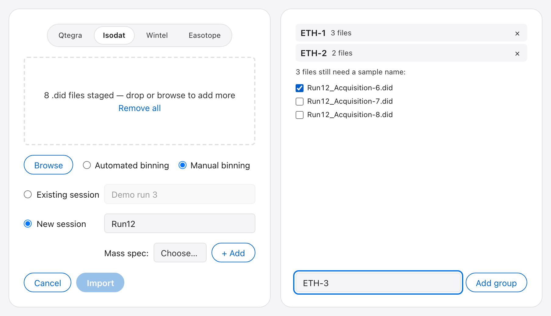
How to bin by hand:
- Tick the files that belong to one sample.
- Type the sample name in the box at the bottom.
- Click Add group. The group appears at the top with its number of files.
- Repeat until the panel says "All files assigned."
The × on a group removes it, and its files go back to the list. Import stays greyed out until every file is in a group.
Easotope database
Use this tab to bring data over from an Easotope database.
Before you start:
- Close Easotope. An open Easotope locks the database, and DELTALab then says so.
- You do not need Easotope or Java installed. DELTALab brings its own.
Steps:
- Drop the Easotope
.h2.dbfile, or the folder that holds it, on the drop area. Or click Browse and choose the file. After an import, DELTALab remembers the file for next time. - Click Analyze. This is a safe trial run: nothing is written yet. A second panel opens on the right and lists every session DELTALab found.
- For each session, check the name, the isotope system and the mass spectrometer. Change them if needed. Untick any session you don't want.
- Click Import in the right-hand panel. DELTALab takes a safety backup first (chapter 8), then brings in the ticked sessions.
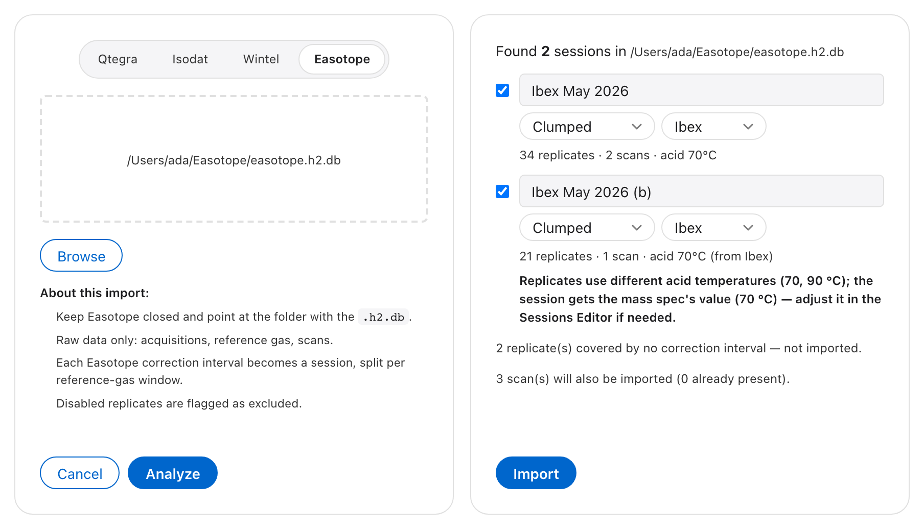
If Analyze shows a message in place of the list:
- "the Easotope database is locked — close Easotope and retry": Easotope is still open. Close it and click Analyze again.
- "no *.h2.db file found in …": the folder you chose holds no Easotope database.
- "found more than one *.h2.db file in …": choose the database file itself, not the folder.
- "Found 0 sessions": the database holds no replicate that is inside a correction interval.
How DELTALab builds the sessions:
- Each Easotope correction interval becomes one session.
- An interval is split wherever the reference gas changes. The second part gets "(b)" after its name, the third "(c)".
- A replicate that is in no correction interval is not imported. The panel says how many there are.
What each session's line tells you:
- the number of replicates and scans;
- how many replicates are already imported, if any. They are skipped, so importing the same database again is safe;
- the acid temperature the session will get. "(from …)" or "(built-in default)" means the value does not come from Easotope.
- A line in bold is a warning. Read it before you import.
What comes across:
- Only raw acquisitions, reference gas and scans are imported. Easotope's own corrected or standardised values are not. DELTALab recalculates everything itself.
- Every replicate in a correction interval is imported. Replicates that were disabled in Easotope arrive excluded, and so do disabled cycles (chapter 4.1).
- Reference gas: the values recorded in Easotope for that session.
- Acid temperature: Easotope's value when all replicates of the session agree. Otherwise the session gets the mass spectrometer's value, or 90 °C for an instrument DELTALab does not know yet. If the replicates differ, a warning tells you.
- Mass spectrometer: the one recorded in Easotope is preselected. Every session needs one; a session without one gets a red outline when you click Import. An instrument DELTALab has not seen before is added to Settings → Mass spectrometers (chapter 7) with that session's reference gas and acid temperature.
Choosing the session and the mass spectrometer
On the Qtegra and Isodat tabs, choose where the data goes (4 in the first picture):
- New session: DELTALab suggests a name from the first file. Type your own if you prefer.
- Existing session: the new acquisitions are added to that session. If the suggested name is already a session, DELTALab chooses it for you. Deactivated sessions are not in this list.
Every session must have a mass spectrometer. The Mass spec line (5) is shown when the session has none yet: for a new session, or for an old session imported before mass spectrometers existed.
- Pick the instrument from the menu. If you have only one, it is already chosen.
- The session gets the reference gas and the acid temperature of that instrument, and keeps its own copy of these values. Change them later in the Sessions Editor (chapter 6).
- Another instrument is not added here: the line carries a hint, and new instruments are added in Settings → Mass spectrometers (chapter 7).
Importing the same data twice is safe
DELTALab recognises an acquisition by its date and time. One that is already in the database, in any session, is skipped. So you can import a folder again after adding new files to it: only the new acquisitions come in. The window tells you how many were skipped.
When DELTALab leaves something out
DELTALab never leaves data out silently. This applies to the Qtegra and Isodat tabs.
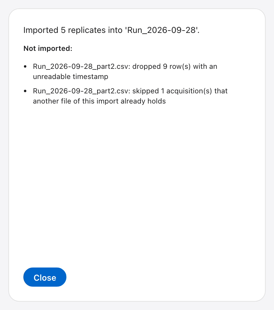
Some data was imported, some was not. The window stays open. It says how many replicates were imported and into which session, and lists under Not imported: everything that was left out, with the reason. Click Close when you have read it.
Nothing was imported. The window stays open with your files still waiting. In red it says "No new, readable acquisitions found.", and below that it gives the reason for each file. Choose Remove all and other files, or Cancel.
The reasons you can see:
| The window says | What it means |
|---|---|
| "… already imported" | These acquisitions (Qtegra) or files (Isodat) are already in the database, in this or another session. |
| "… that another file of this import already holds" | The same acquisition is in two of your files. It was imported once. |
| "dropped … row(s) with an unreadable timestamp" | These rows of a Qtegra file have no date DELTALab can read. |
| "cannot tell whether timestamps … are DD/MM or MM/DD" | The dates of this Qtegra file can be read both ways. The file is refused (see above). |
| "skipped — this batch is being read as …" | This file's dates contradict the other files you chose with it. |
| "doesn't look like a Qtegra export" | The file is not a Qtegra CSV. |
| "could not be read" | The CSV file is damaged or empty. |
| "Skipped … .did: …" | DELTALab cannot read this .did file, or it has no sample cycles. |
| "… sample cycle(s) have no matching reference cycle and were dropped" | The acquisition stopped early. The complete cycles were imported. |
The same list is kept in Session History (chapter 4.3), under the import's own line, so you can read it again after you close the window.
Adding data to a session that is already standardised
Important:the new replicates get a provisional
Δ₄₇straight away, using the session's existing fit. Their uncertainties stay blank and the session gets a red flag. Re-run standardisation (chapter 5) to update everything properly. A session standardised with the Easotope Moving window has no session fit, so its new replicates stay blank until you run it again.
Merging another DELTALab database
Open Import and choose the DELTALab tab. Browse to the other .db file and press
Analyze: every session in that file is listed with what merging would do.
| Label | Meaning |
|---|---|
| New | The session is not in your database. It is copied as it is, with its settings and history. |
| Add N | A session with that name exists. Only the N replicates you do not have yet are added, and they are recalculated with your session's settings. |
| Already here | Every replicate is already in your database. Nothing to do. |
A replicate counts as already there when its acquisition time matches one in your database, whichever session holds it. You can therefore merge the same file again later and only new replicates are added. If a session of the same name was measured on another instrument, the incoming one is added as "name (merged)". The other file is only read, and a backup of your database is taken first. After adding replicates to an existing session, re-run standardisation (chapter 5).
3.1 How to setup QTegra Export
DELTALab reads the raw beam intensities of a Qtegra export and works out the deltas itself (chapter 3, "Qtegra (CSV files)"). So the export must hold the intensities and a few identifying columns. You set this up once in Qtegra's Query page and save it as a preset, and every later export is two clicks.
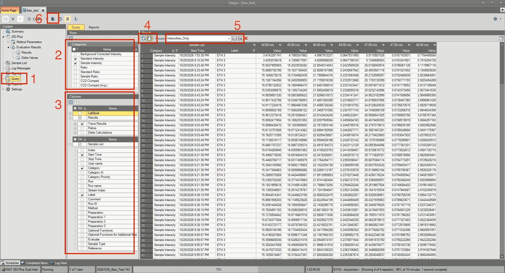
- Open the Labbook you want to export and click Query in the list on the left.
- Under the tab called "Categories", select only Standard Intensity and Sample Intensity.
- In the Columns section:
- Under Sample List, tick Start Time, Category and Label.
- Under Results, tick Trace Results.
- Click the reload button (the circle made of two arrows) to load the data with the structure you defined. Then click the weight button, next to the reload button, to remove the measuring unit from the table. The table should now have one row per cycle: the category, the start time, the label (your sample name), and one intensity per mass.
- Presets. When the table looks like the one in the picture, save it under a name (here Intensities_Only) with the save button next to the box. Next time, choose the preset and the categories and columns are set for you.
-
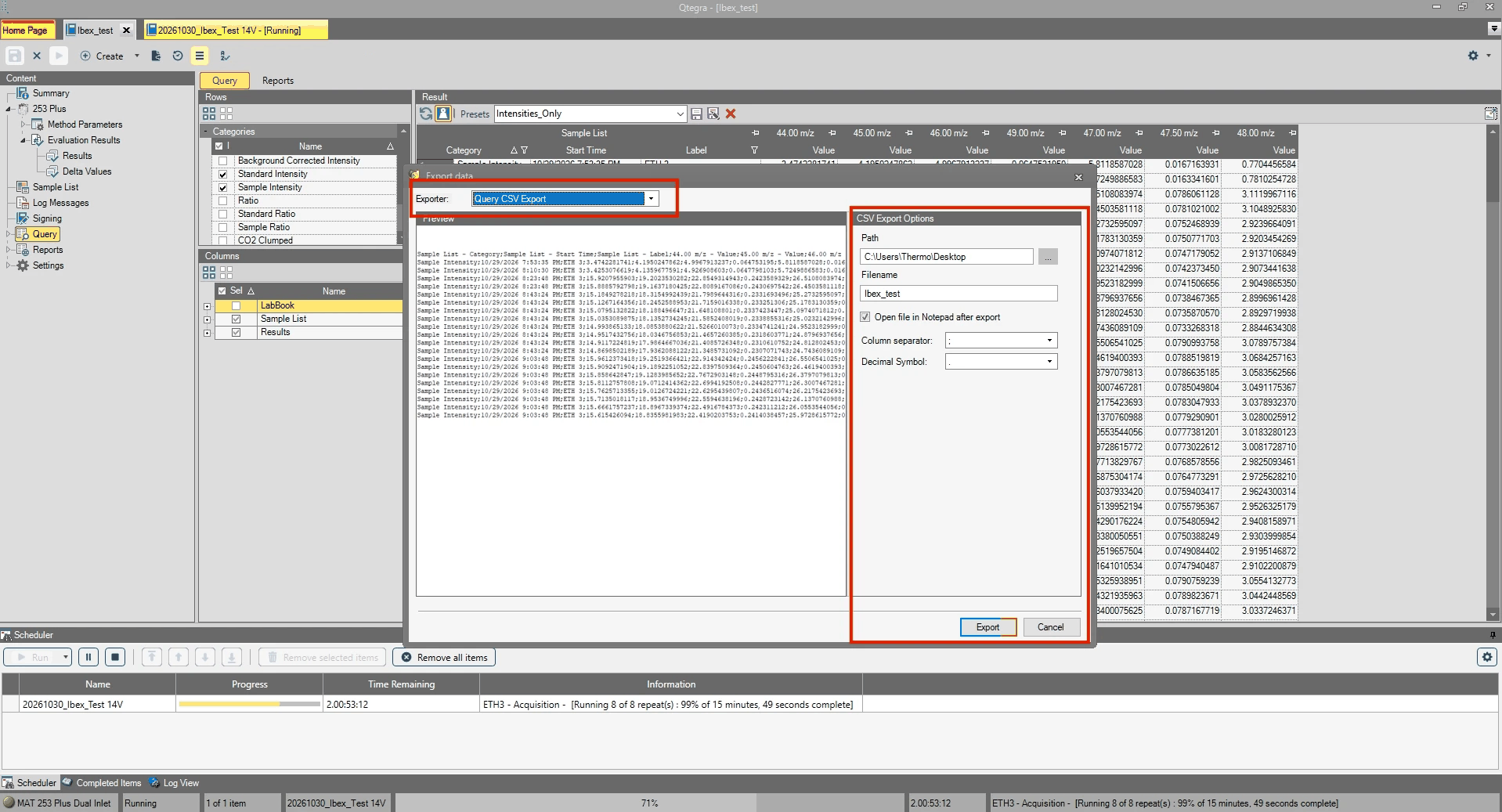
Click Export data in the toolbar. The export window opens.
-
Set Exporter to Query CSV Export.
- Under CSV Export Options, choose the Path (the folder) and the Filename.
Set the Decimal Symbol to a point (
.): DELTALab does not read numbers written with a decimal comma. - Click Export.
4. The Explore page
The Explore page is where you look at your data: the plots, the tables and the log of the sessions you selected. DELTALab opens on this page.
You do not process data here. Processing happens on the Standardization page (chapter 5); the Explore page shows you the result. The only things you change here are exclusions and attachments (chapter 4.1) and notes in Session History (chapter 4.3).
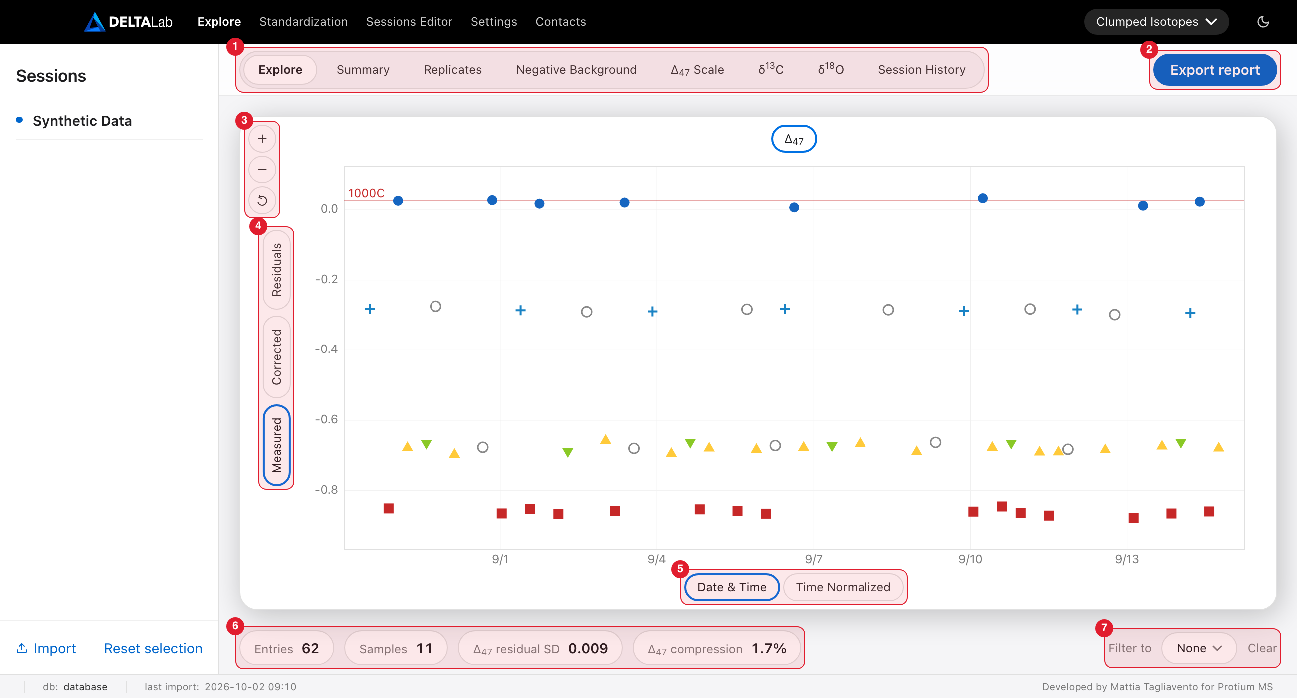
Marked in red: 1 the tabs, 2 Export report, 3 the zoom buttons, 4 the value buttons, 5 the time-axis buttons, 6 the summary bar, 7 Filter to.
What decides what you see
Three choices, in this order:
- The sessions selected in the session list (chapter 2). Every selected session is shown together, merged. With no session selected every tab says "Please select a session".
- The isotope-system menu in the top bar. It decides which tabs the page has.
- The tab you click (1 in the picture).
Same name twice:Explore in the top bar is the whole page. Explore in the row of tabs is its first tab, the plot against time.
The tabs of each isotope system
- Clumped Isotopes: Explore · Summary · Replicates · Negative Background · Δ₄₇ Scale · δ¹³C · δ¹⁸O · Session History.
- Dual Clumped: Explore · Summary · Dual Equilibrium · Replicates · Negative Background · Δ Scales · δ¹³C · δ¹⁸O · Session History. Δ₄₈ is shown next to Δ₄₇ throughout.
| Tab | What it shows |
|---|---|
| Explore | Every replicate against time |
| Summary | One row per sample: averages, uncertainties and temperature |
| Replicates | One row per replicate; you exclude measurements here |
| Dual Equilibrium | Δ₄₇ against Δ₄₈ with the equilibrium curve (Dual Clumped only) |
| Negative Background | A check of the background correction |
| Δ₄₇ Scale, Δ Scales | Measured or corrected Δ against the accepted values |
| δ¹³C, δ¹⁸O | One tab per isotope: the plot against time and its scale plot (Overview / Scale) |
| Session History | The log of everything done to the selected sessions |
The sections below follow the same order.
The Explore tab: Δ against time
One point per replicate, with Δ₄₇ on the vertical axis and time on the horizontal axis. Use it to see a whole run at a glance: drift, jumps, outliers, and how well the standards agree with their accepted values.
The value buttons (left of the plot, 4 in the picture):
- Measured:
Δ₄₇ raw. The plot opens on this view. - Corrected: the standardised Δ₄₇.
- Residuals: how far each point sits from the standardisation fit, around a zero line. Use it to judge the fit and to spot a drifting session.
Corrected and Residuals need a standardisation. Until you have run one, every point sits on a flat line at zero. After a run, Go to Explore on the Standardization page opens this plot directly on Corrected.
The button above the plot names the Δ you are looking at. On Dual Clumped there are two, Δ₄₇ and Δ₄₈, and they switch between the masses.
The time-axis buttons (under the plot, 5 in the picture):
- Date & Time: real dates, with gaps where nothing was measured.
- Time Normalized: measurement order, with equal spacing. Thin lines mark where one session ends and the next begins.
Reading the plot:
- Standards are filled, coloured markers. Each standard has its own colour and shape, set in the Marker column of Settings → Reference material (chapter 7).
- Unknown samples are open grey circles.
- Excluded replicates stay on the plot, pale grey, so you can still see where they were.
- Coloured horizontal lines mark each standard's accepted Δ, with its name at the left
end. A line is only drawn when its value falls inside the range of the plot.
- In Corrected, each standard should scatter around its own line.
- In Measured, the points do not sit on the lines. Raw values are not on the reference frame yet, so most lines fall outside the plot.
- In Residuals, there is one zero line instead.
- Hover over a point to see its sample, session, ID, date and value.
The size of the points is set by Marker size in Settings → Display preferences.
Important:a standard only counts as a standard on this page if its Show in plots box is ticked for the isotope system you are in (Settings → Reference material). With the box unticked it is drawn, counted and filtered like an unknown sample. This has no effect on which standards a fit uses.
The Summary tab
One row per sample, in alphabetical order. Excluded replicates are left out; n is the number of replicates that remain.
- δ¹³C, δ¹⁸O: the sample averages. A δ¹⁸O AF column appears after δ¹⁸O as soon as any replicate in view has an acid-fractionation-corrected value (chapter 5.1).
- Δ₄₇: the sample's standardised value, calculated the same way as D47crunch's sample table. It is not just the average of the replicates. Before standardisation, it shows the average instead.
- SE: standard error, including both the measurement and the standardisation uncertainty.
- 95 % CL: 95 % confidence limit (SE × Student's t).
- SD: how much the sample's replicates scatter (standard deviation, n − 1).
- T, T SE: the average temperature and the average temperature uncertainty.
Dual Clumped adds Δ₄₈ with its own SE, 95 % CL and SD.
A small coloured dot after δ¹³C, δ¹⁸O, δ¹⁸O AF, Δ₄₇, Δ₄₈ and T says whether that value can be used as it is: green, yellow, orange or red. Chapter 4.4 explains the colours and what to do about each.
SE and SD are different things. SE is the calculated uncertainty. SD is how much your replicates actually scatter. A sample with a single replicate has no SD ("—"), so SE is its only error bar. Do not calculate SE as SD ÷ √n; that gives a different, wrong number.
The Summary always lists every sample of the selected sessions. It ignores Filter to.
The Replicates tab
One row per replicate. The columns are, from left to right:
- QC: a round dot. Click it to exclude or include the replicate (chapter 4.1).
- Paperclip: files and a note attached to this replicate (chapter 4.1).
- ID
- Date & Time
- Sample: click it to open the raw cycles in the acquisitions window (chapter 4.1).
-
δ¹³C, δ¹⁸O: the δ¹⁸O header is a menu that picks which δ¹⁸O the column shows:
- δ¹⁸O (default): standardised δ¹⁸O. "—" until Bulk Standardization has run.
- δ¹⁸O raw: the value from import, never standardised.
- δ¹⁸O AF: the mineral δ¹⁸O from the acid fractionation correction (chapter 5.1). "—" for samples not corrected.
Your choice stays when you switch tabs or isotope systems.
-
Δ₄₇ raw. Dual Clumped also has Δ₄₈ raw.
- Δ₄₇: standardised Δ₄₇. Dual Clumped also has Δ₄₈.
- Δ₄₇ SE: the sample's standard error from standardisation, repeated on each of its replicates.
- T (°C), T SE: temperature and its uncertainty.
δ¹³C and δ¹⁸O show the standardised value once Bulk Standardization has run, and the raw value until then. Hover over a standardised value to see the raw value behind it.
A cell shows "—" when there is no value yet:
- Δ₄₇ and Δ₄₇ SE need standardisation (chapter 5).
- T (°C) needs temperature conversion.
- T SE needs temperature conversion with Propagate calibration uncertainties ticked.
The Dual Equilibrium tab (Dual Clumped only)
Plots Δ₄₇ against Δ₄₈ together with the theoretical equilibrium curve. The numbers along the curve are temperatures in °C.
- Replicates shows one point per replicate.
- Summary shows one point per sample. Hover over it to see how many replicates it averages.
Samples that plot away from the curve point to kinetic effects or a correction problem.
Filter to decides what is drawn: set it to Samples to hide the standards.
The Negative Background tab
Plots Δ₄₇ (vertical) against δ₄₇ (horizontal) for your standards, with one regression line per standard group and a shaded 95 % confidence band around it. On Dual Clumped the Δ₄₇ and Δ₄₈ buttons switch to the mass-48 pair.
A good background factor makes these lines flat. Use the plot to check the minimizer's result, or to judge a fixed factor by eye (chapter 5).
- Gas and Carbonates choose which family of groups is shown.
- Measured and Corrected choose which Δ value is plotted.
- The groups come from the Neg. Bkg eval. column of Settings → Reference material. If no standard has a group, the plot says "No standard groups defined".
This plot always uses all standards. It ignores Filter to.
The Δ₄₇ Scale tab (Clumped) and Δ Scales tab (Dual)
Plots each standard's Δ (vertical) against its accepted Δ (horizontal, Expected), with a fitted line. The equation of the line and the uncertainty of its slope are printed on the plot. On Dual Clumped the Δ₄₇ and Δ₄₈ buttons switch masses.
- Until you standardise, the tab says "Standardise this session to visualize this plot".
- Measured plots raw Δ and Corrected the standardised Δ.
- A Measured slope below 1 means scale compression. The Δ₄₇ compression value in the summary bar gives it as a percentage.
- The plot shows the standards the session was standardised with. Add to the plot, which takes the place of Filter to on this tab, adds other reference materials. An added material is drawn and also counts in the fitted line. All ticks every one of them, and Clear removes them again.
- Hover over a point to see its expected value, its raw value and the difference.
This plot always uses the full data set of the selected sessions.
The δ¹³C and δ¹⁸O tabs
Each tab holds two plots, switched with the Overview and Scale buttons at the top.
Overview is the isotope against time. It works like the Explore tab's plot, with two differences: the value buttons are only Measured and Corrected (after Bulk Standardization), and there is no Residuals view.
Scale plots each standard's value against its accepted value, with a fitted line, as on the Δ₄₇ Scale tab. It needs Bulk Standardization, and it shows the standards that run used. Measured and Corrected choose the vertical axis.
On these two tabs, a standard counts as a standard when the Bulk box of its Show in plots column is ticked (Settings → Reference material). The equilibrated gases have no bulk values and no Bulk tick, so they are drawn as open grey circles.
The coloured horizontal lines mark where each reference material is expected.
- For δ¹⁸O that value depends on the acid reaction temperature: the carbonate's δ¹⁸O is converted to the CO₂ it releases. Each session has its own temperature, taken from its mass spectrometer.
- When the sessions you plot were run at different temperatures, each material gets one line per temperature. The lines for the first temperature are solid with their labels on the left. The lines for the other temperatures are dashed with their labels on the right.
- Every label shows its temperature, for example
ETH 3 (70 °C).
The δ¹⁸O plot shows the standardised δ¹⁸O, not δ¹⁸O AF.
The Session History tab
The permanent log of the selected sessions, newest first. See chapter 4.3.
Zooming and panning plots
- Use the +, − and ⟲ (reset) buttons at the top left of a plot (3 in the picture).
- On a trackpad, pinch to zoom. With a mouse, hold Ctrl and turn the wheel.
- Click and drag across a plot to draw a rectangle; the plot zooms in to that area.
- Once zoomed in, hold Shift and drag to move around, or scroll with two fingers.
- Hover over a point to see its details.
Changing a plot's value buttons or its time axis resets the zoom.
The summary bar
The bar at the bottom of the Clumped and Dual pages (6 in the picture) summarises the selected sessions.
- Entries: the number of replicates. This is the only number that still counts excluded replicates.
- Samples: the number of replicates that belong to unknown samples, not to standards. Excluded replicates are not counted.
- Δ₄₇ residual SD: the scatter (standard deviation) of the residuals, the same values the Residuals view plots. Smaller is better. "—" until you standardise.
- Δ₄₇ compression: how far the slope of raw Δ against the standards' accepted Δ is from 1, as a percentage.
Dual Clumped adds Δ₄₈ residual SD and Δ₄₈ compression.
These numbers always describe all replicates of the selected sessions. Filter to does not change them.
Filter to
Filter to (on the right of the summary bar, 7 in the picture) narrows what you see. It never changes a calculation.
Click the button to open the menu:
- None: show everything. This is what the page opens on.
- Standards: show only the standards.
- Samples: show only the unknown samples.
- Below the line: tick individual samples. As soon as one is ticked, the button reads "N selected" and only the ticked samples are shown. Clear unticks them and goes back to None, Standards or Samples, whichever was chosen.
What the filter applies to:
| Follows the filter | Ignores the filter |
|---|---|
| Explore plot | Summary |
| Replicates | Negative Background |
| Dual Equilibrium | Δ₄₇ Scale, Δ Scales |
| δ¹³C and δ¹⁸O Overview plots | δ¹³C and δ¹⁸O Scale plots |
| Session History | |
| The numbers in the summary bar |
Summary always lists every sample, and the diagnostic plots always use the full set of standards.
The filter stays while you move between tabs. It goes back to None when you leave the Explore page or change the isotope system.
Export report
Export report (top right, 2 in the picture) saves the tables and plots of the selected sessions to files. See chapter 4.2.
4.1 Checking raw data and excluding bad measurements
You do all of this on the Explore page, in the Replicates tab (chapter 4 describes the page and every column of the list).
Three things in each row of the list matter here:
- the QC dot at the start of the row, which excludes or includes the replicate;
- the paperclip, which opens its attachments;
- the Sample name, which opens its raw cycles.
The acquisitions window: raw cycles
Click a Sample name to see the raw voltages behind that replicate.
- The buttons on the left (Acq. 1, Acq. 2, …) choose the acquisition.
- Each row of the table is one cycle, showing the sample and reference voltages from V44 to V49, plus V47.5 where you have it.
- Under the table are the Δ₄₇ raw of the chosen acquisition and the internal SD: the scatter of the Δ₄₇ raw of this replicate's acquisitions. Dual Clumped adds the same for Δ₄₈. The internal SD counts applied exclusions only, so "(before Apply)" tells you the numbers do not include your latest clicks yet.
- For Isodat
.didfiles with a logged reading, two labels above the table give the left and right bellows pressure and position from the moment Isodat skipped the reference refill.
Use this window to look into a suspicious replicate. You can also exclude part of a replicate here, instead of the whole thing.
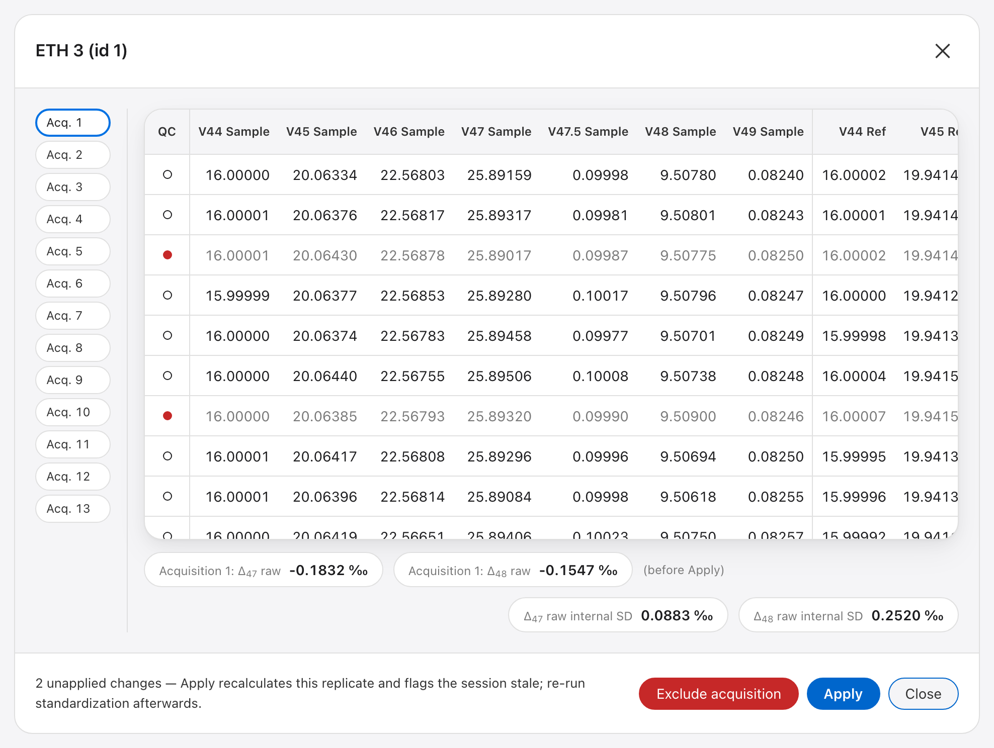
Cycles 3 and 7 are marked for exclusion (red dot, greyed values). Nothing changes until you click Apply.
To exclude single cycles:
- Click the QC dot at the start of each bad cycle.
- Click Apply. DELTALab recalculates that replicate from the cycles that are left, and marks the session as out of date. Re-run standardisation afterwards.
To exclude a whole acquisition:
- Click its Acq. button.
- Click Exclude acquisition, then Apply. (On a fully excluded acquisition the button reads Include acquisition.)
Good to know:
- Changes wait until you click Apply. If you close the window with changes still waiting, DELTALab asks whether to throw them away.
- You cannot exclude every cycle of a replicate here. To remove the whole replicate, use its QC dot in the Replicates.
- Cycle and acquisition exclusions are recorded in Session History (chapter 4.3).
Excluding a whole replicate
Click the QC dot at the left of the row. An excluded replicate:
- is left out of the Summary, of every fit (background, standardisation, scale compression, temperature) and of the Samples count;
- stays visible, greyed out, in the Replicates and the acquisitions window, so you can always see it and change your mind;
- stays excluded when you re-process, edit the reference gas, re-import or move it to another session.
Excluding or including a replicate marks the session as out of date (red flag). Re-run standardisation afterwards.
Attachments: files and notes on a replicate
Click the paperclip in a replicate's row to keep files and a note with that replicate. Examples: a lab-book photo, an instrument log, a weighing sheet.
- Attach files:
.csv,.jpg,.xlsxor.pdf. CSV files and Excel sheets can be previewed in the window (the first 50 rows × 26 columns); a PDF is opened with Save a copy. - Add comment: one free-text note per replicate.
- Save a copy downloads an attached file or the note. Delete removes it.
- One replicate can hold up to 3 files and 5 MB in total, note included.
4.2 Exporting a report
Export report saves the tables and plots of the sessions you selected as files: tables as CSV, plots as PDF. Use it to archive a result, to work on the numbers in another program or to send data to a colleague.
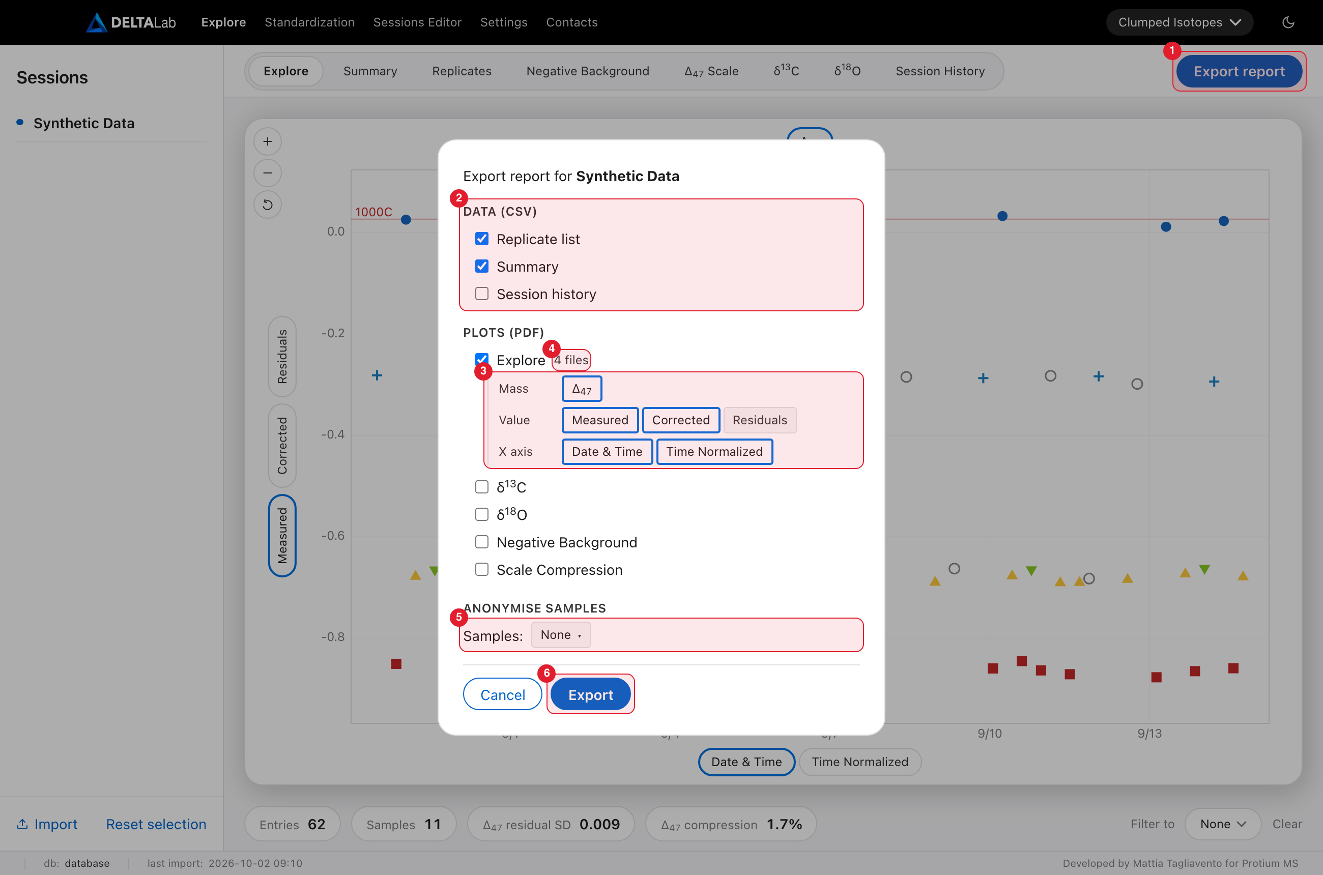
Marked in red: 1 Export report, 2 the tables, 3 a plot's options, 4 the number of files, 5 Anonymise samples, 6 Export.
How to export
- On the Explore page (chapter 4), select the session or sessions in the session list.
- Click Export report (1). The title of the window names the sessions.
- Tick the tables (2) and the plots you want.
- For each ticked plot, choose its options (3).
- Optionally hide sample names with Anonymise samples (5).
- Click Export (6).
If Replicate list or Summary is ticked and some of its values do not have a green dot, a warning opens before the files are written (chapter 4.4).
Good to know:
- The export covers every replicate of the selected sessions. The Filter to menu of the Explore page does not apply.
- Deactivated sessions are never exported. The window lists them under "Left out (deactivated)".
- The isotope system in the top bar decides which columns and plots are offered.
- The window starts empty every time you open it. Nothing is ticked and the options are back to their starting values.
- With nothing ticked, Export tells you to select at least one item. With no session selected, the window asks you to select one and open it again.
- An export changes nothing in your data and is not written to Session History (chapter 4.3).
The tables (CSV)
- Replicate list: one row per replicate, with the same values as the
Replicates tab, plus the raw δ⁴⁵–δ⁴⁹ and the
Excludedflag. Excluded replicates are kept, as on screen. - Summary: one row per sample with the number of replicates and the mean and SD of each value, as in the Summary tab. Excluded replicates are left out, and so is a sample whose replicates are all excluded.
- Session history: the log of the selected sessions, one row per entry, with its date, its kind, its description, its full details and any note.
Good to know:
- A value that does not exist yet is left empty, for example a temperature before Temperature Conversion, or δ¹⁸O AF before the acid correction.
- Replicate list and Summary have no session column. With several sessions selected, their replicates are listed together and the Summary reports each sample over all of them (chapter 4.4 says how Δ values from several standardisations are combined). Export one session at a time if you need to keep them apart. The Session history file does name the session of each entry.
- Bulk values in the Summary are the standardised ones when they exist, and the raw ones otherwise.
The plots (PDF)
Explore, δ¹³C, δ¹⁸O, Negative Background and Scale Compression. They are the same plots as on the Explore page, with the same look. Scale Compression is the measured plot of the Δ₄₇ Scale tab (Δ Scales on Dual Clumped).
Ticking a plot shows the same choices as the plot on screen:
| Plot | Choices |
|---|---|
| Explore | Mass; Value: Measured, Corrected, Residuals; X axis: Date & Time, Time Normalized |
| δ¹³C, δ¹⁸O | Value: Measured, Corrected; X axis: Date & Time, Time Normalized |
| Negative Background | Mass; Value: Measured, Corrected; Groups: Gas, Carbonates |
| Scale Compression | Mass |
- Click a choice to add it or remove it. One choice in each row always stays on. Each plot starts on Measured and Date & Time.
- Each combination is a separate figure. Measured and Corrected, each against Date & Time and Time Normalized, makes four. The note next to the plot (4) tells you how many files that plot will give.
- Groups is the exception: the groups you choose are drawn side by side in one figure.
- A figure shows all selected sessions together.
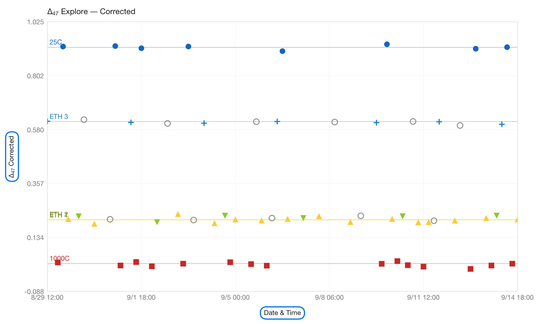
An exported figure: Explore, Corrected against Date & Time. Standards keep their marker and colour from Settings; samples are open grey circles.
Anonymise samples
Use this to share data without showing what your samples are.
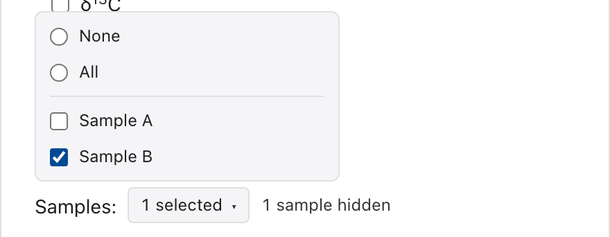
- Click the Samples menu.
- Tick the samples to hide, or choose All. None clears the choice.
- Click outside the menu to close it. The text next to the menu says how many samples are hidden.
What happens in the export:
- Each hidden sample is renamed Unknown 1, Unknown 2, … in the order they were first measured. Samples you did not tick keep their names.
- The same sample gets the same label in every file of that export: the tables, every plot and the Session history.
- Standards are never renamed and are not in the list. Their values are published.
- Only the exported files are changed. The names in DELTALab stay as they are.
The files you get
- One item ticked: that file, a
.csvor a.pdf. - Several items, or one plot with several figures: a single
.zipwith all the files in it.
File names start with the session name, with spaces and special characters
replaced by _. With several sessions selected they start with export
instead.
| Item | File name, for the session "Synthetic Data" |
|---|---|
| Replicate list | Synthetic_Data_Replicate list.csv |
| Summary | Synthetic_Data_Sample summary.csv |
| Session history | Synthetic_Data_Session history.csv |
| Explore | Synthetic_Data_Data Explore (D47 corrected vs Date).pdf |
| δ¹³C, δ¹⁸O | Synthetic_Data_d13C (raw vs Date).pdf, Synthetic_Data_d18O (raw vs Date).pdf |
| Negative Background | Synthetic_Data_Negative background (D47 raw).pdf |
| Scale Compression | Synthetic_Data_Scale Compression (D47).pdf |
| Everything together | Synthetic_Data_export.zip |
The name of a plot file says which figure it is.
Dual Clumped
With Dual Clumped chosen in the top bar:
- the Replicate list also carries the Δ₄₈ residual, the sample's Δ₄₈ and its uncertainties;
- Mass offers Δ₄₇ and Δ₄₈ for Explore, Negative Background and Scale Compression. Choosing both doubles the figures;
- one more plot is offered, Dual Equilibrium, with the choice View: Replicates or Summary.
4.3 Session History
Session History is a permanent log of what happened to each session. Entries are only ever added, never changed, though you can add a note to any of them. It records:
- imports;
- excluding and including replicates, cycles and acquisitions;
- background corrections;
- standardisations, temperature conversions and acid fractionation corrections;
- changes made in the Sessions Editor (chapter 6):
- renaming a session;
- changing its mass spectrometer, reference gas or acid reaction temperature;
- splitting a session;
- deactivating and activating a session;
- moving, renaming and deleting replicates.
Open the Session History tab of the Explore page (chapter 4). It shows every selected session together, newest first.
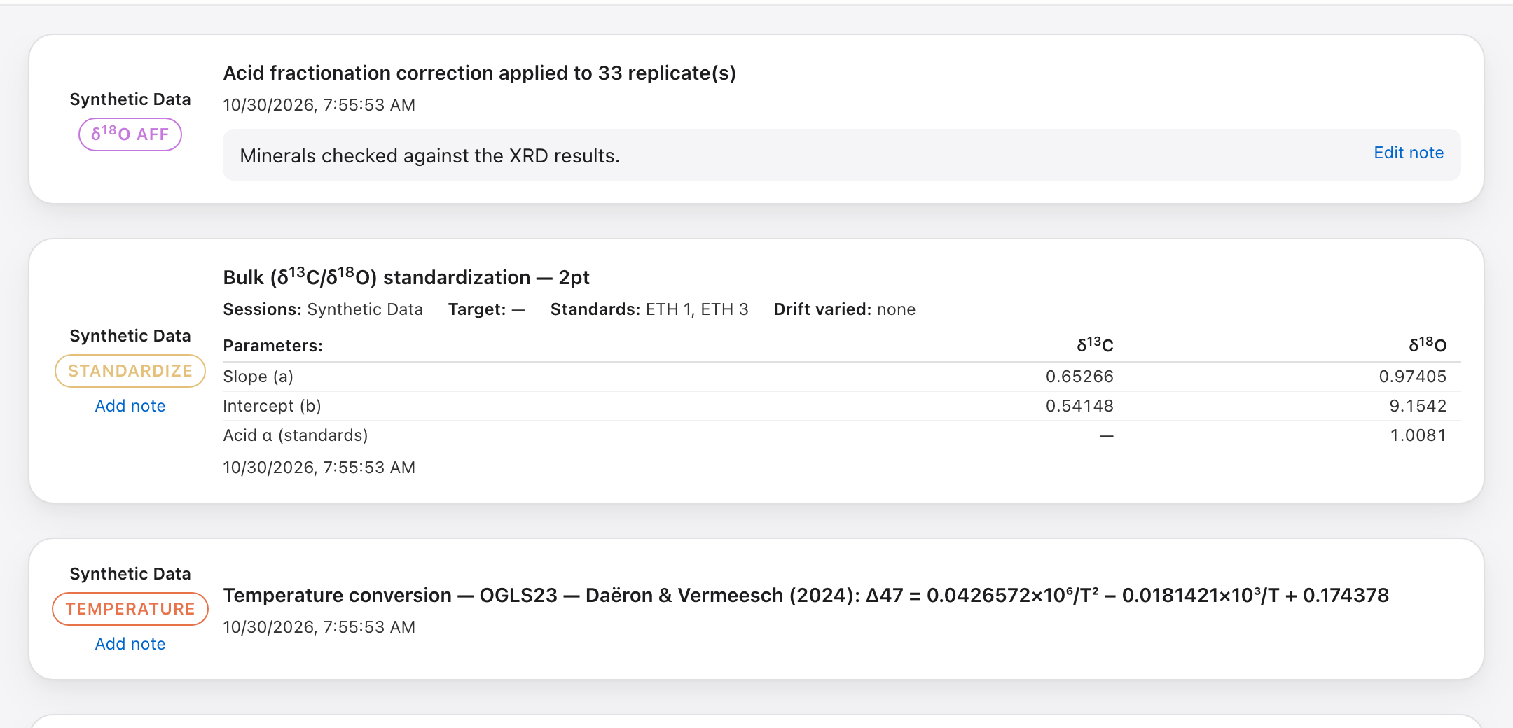
- An import entry says how many replicates came in. If the import left something out, the entry lists it under "Not imported:", with the reason (chapter 3).
- Click a standardize entry to see everything about that run: the sessions, the target, the standards, the drift terms and the fitted parameters. This is a complete record of how a number was produced.
- Several quick exclude/include clicks in a row are shown as one line. The log itself keeps every click.
- Each entry has a coloured label that says what kind of change it is. Changes to the reference gas, the mass spectrometer and the acid reaction temperature, and moved replicates, carry the Background label, like the background corrections. Deactivating and activating a session carry Deactivated and Activated.
- Add note, under an entry's label, keeps a note of up to 2,000 characters with that entry, for example why you ran a step again. Edit note changes it; saving it empty removes it. Notes are also in the Session history file of an export.
How Sessions Editor changes appear:
- A renamed session keeps its history. The rename is one more entry.
- A split is written to every part. The part that kept the original name keeps the whole history. Each new session starts with a single entry that says which session it was split from.
- A move is written to both sessions.
- A renamed or deleted replicate is written to its session.
- Deleting a session deletes its history. Nothing about that session is left in the log.
Not recorded: exports, attachments, backups and restores.
4.4 The traffic light
The traffic light is the small coloured dot after each reported value in the Summary tab (chapter 4). It answers one question: can this value be reported as it is, for the replicates I selected?
It appears after δ¹³C, δ¹⁸O, δ¹⁸O AF, Δ₄₇, Δ₄₈ and T. A value that does not exist yet has no dot. Triple Oxygen has no traffic light.
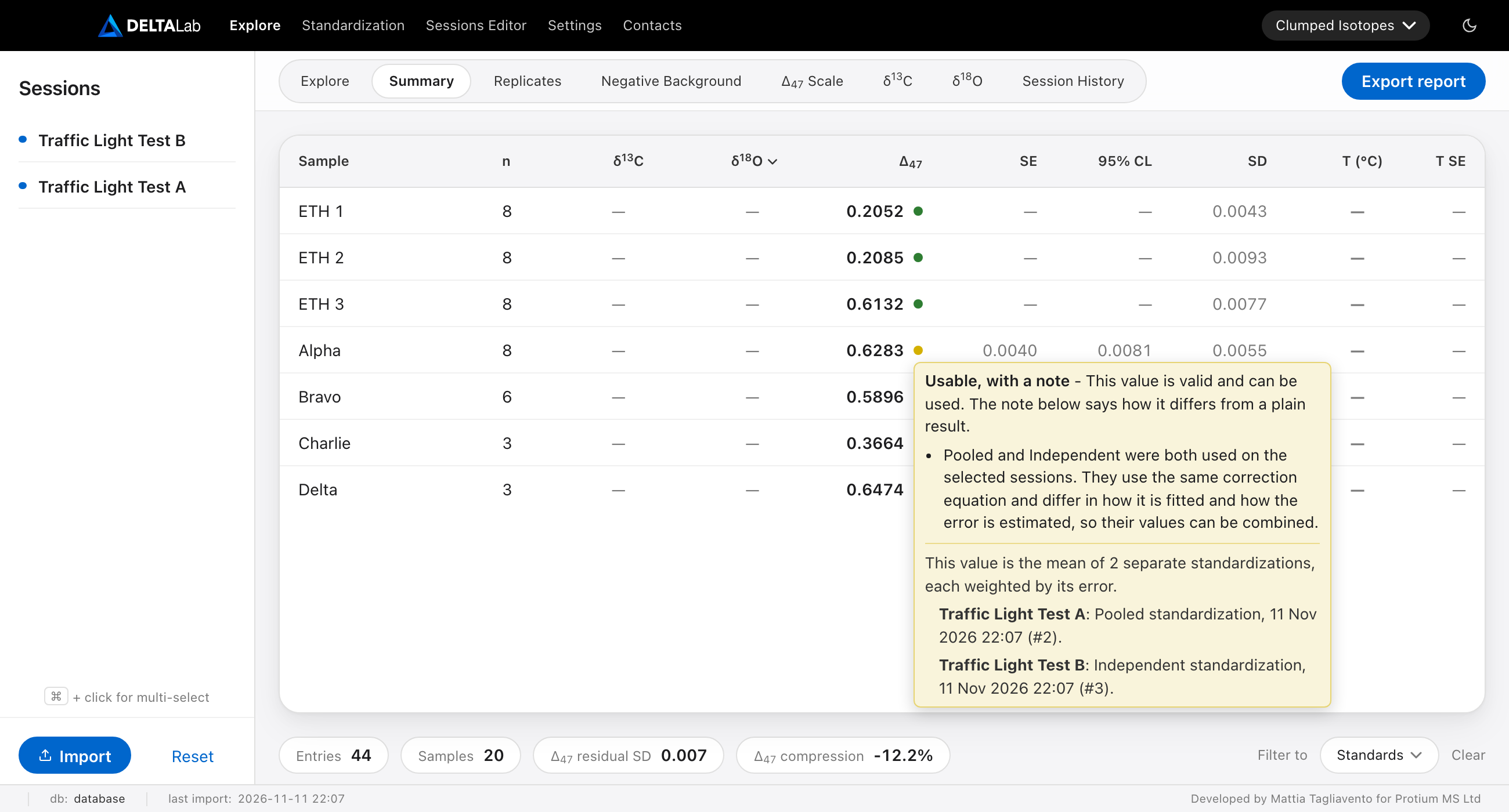
The four colours
| Colour | Headline in the app | Meaning | What to do |
|---|---|---|---|
| Green | Ready to report | The value was calculated from exactly the replicates you selected, and it is up to date. | Nothing. |
| Yellow | Usable, with a note | The value is valid and up to date, but it is not exactly what the selection shows. | Read the note. |
| Orange | Needs an update | The value is out of date or incomplete. | Redo the step the tooltip names. |
| Red | Cannot be reported | It is not mathematically allowable to report one value for these replicates. | Standardise the selected sessions together. |
When a value has several problems, the most serious one decides the colour, and it is listed first.
Reading a dot
- Point at a dot to see why it has that colour: a headline, the reasons, then notes on how the value was produced.
- Click a dot to keep its tooltip open, so you can select and copy the text. Click the dot again, click elsewhere or press Esc to close it.
- Reference entry in the tooltip is a link while the tooltip is kept open. It opens Session History (chapter 4.3) on the entry of the standardisation behind the value.
Why the selection matters
A standardisation writes one value per sample for all the sessions it was run on. The Summary then shows that value for whatever sessions you select. The two do not always match:
- You standardised sessions A and B together, and select only A. The value of a sample measured in both still contains B's replicates.
- You standardised A and B separately, and select both. There are two values for the same sample.
The traffic light tells you which case you are in, and whether it is a problem.
This chapter calls each click of Apply on the Standardization page a run. The
app's tooltips say "standardization"; the export calls them Standardization runs
and numbers them (#4).
Several standardisations behind one Δ value
When the selected replicates of a sample were standardised in separate runs, DELTALab checks whether their values may be combined. They may when all of this is true:
- No session is shared between the runs. Each value then comes from its own measurements of the standards, so the values are statistically independent.
- The runs used the same standards.
- Each standard had the same accepted value in every run.
- Each run produced an SE.
If so, the Summary shows the weighted mean of the runs' values. Each value counts in proportion to its precision:
w = 1 / SE²
Δ = Σ(w · Δ) / Σw
SE = 1 / √(Σw)
95 % CL = SE × t, with Student's t for the combined degrees of freedom
(Welch–Satterthwaite).
- Two runs with the same SE give the plain average, with an SE smaller by √2.
- This is the calculation Independent standardisation does inside one run (chapter 5).
- The tooltip says "This value is the mean of 2 separate standardizations, each weighted by its error." and names each one.
- Nothing is stored: the combined value is calculated from the stored values every time, on screen and in the exported Summary alike.
Runs with different settings combine too: different drift terms (Pooled, Independent) or different Easotope ETF options. These are chosen for each session, as in D47crunch, and the tooltip adds a note that says so.
If one of the four conditions fails, the dot is red. The Summary then shows the value of the first run only, so do not use it for the whole selection.
Red: what makes a value not allowable
Δ₄₇ and Δ₄₈: the tooltip lists every problem that applies, one sentence each, in the order of the table, followed by one line per standardisation. A second problem is therefore not hidden behind the first.
| The tooltip says | Why it is not allowable |
|---|---|
| "Session B is part of more than one of these standardizations, so its data would be counted twice in the average…" | Both values contain session B's data. They are not independent, and averaging them would count B twice. |
| "These standardizations did not use the same standards (ETH 2 was not used in all of them)…" | Different standards define different reference frames. |
| "The accepted value of ETH 3 was not the same in these standardizations…" | The values are on different scales. |
| "One of these standardizations reported no error (SE) for this sample…" | Without an SE a value cannot be weighted. |
| "One of these standardizations did not record the accepted values of its standards…" | The reference frame cannot be checked. Standardise again. |
- A standard shows its accepted value, so it is green whatever you select. It turns red only if it had different accepted values in the selected runs.
- A material that is a standard in one session and an unknown in another is red.
The other values:
| Value | Red when |
|---|---|
| δ¹³C, δ¹⁸O | the replicates were bulk-standardised in separate runs |
| T | the replicates were converted with different calibrations |
| δ¹⁸O AF | the replicates were corrected with different minerals or constants |
Temperatures converted in separate runs with the same calibration are green. So are mineral values corrected in separate runs with the same mineral.
To clear a red dot, run the step again on the selected sessions together (chapter 5).
Orange: redo a step
| The tooltip says | Applies to | What to do |
|---|---|---|
| "Session A has changed since it was standardized (2 replicates added)…" | Δ, δ¹³C, δ¹⁸O | Standardise the session again. The change can be replicates added, removed, renamed or recalculated, or exclusions changed. |
| "1 of 8 replicates was added or changed after the standardization, so it has no standardized value…" | Δ | Standardise the session again to include it. |
| "Easotope ETF and Pooled do not use the same correction equation…" | Δ, combined runs | Treat the combined value with caution. This is an Easotope ETF run combined with a Pooled or Independent one: the correction equations differ. |
| "…have not been bulk-standardized yet, so this average mixes corrected and uncorrected values." | δ¹³C, δ¹⁸O | Run Bulk Standardization on those sessions. |
| "…standardized again after the Temperature Conversion, so it has no temperature yet and is not part of this average." | T | Run Temperature Conversion again. |
| "…bulk-standardized again after the Acid Fractionation Correction, so it has no mineral δ18O yet and is not part of this average." | δ¹⁸O AF | Apply the acid fractionation correction again. |
With several sessions selected, a message that counts replicates names the sessions they are in: "4 of 11 replicates (session B) were standardized again after the Temperature Conversion…". With one session selected the name is left out.
Undoing the change also clears "has changed", for example including again the replicate you excluded. It is the same rule as the red flag of the session list (chapter 2).
Yellow: usable, with a note
A yellow value can be reported. Read the note, so you know what the value covers.
| The tooltip says | Applies to | Meaning |
|---|---|---|
| "This value is valid, but its standardization also used sessions that are not selected: B." | Δ | The value includes this sample's replicates in a session you did not select (after Pooled: any other session of that standardisation). It is correct, but n and SD in the row cover only the selection. Select B too to see everything behind the value. |
| "Pooled and Independent were both used on the selected sessions. They use the same correction equation and differ in how it is fitted and how the error is estimated, so their values can be combined." | Δ, combined runs | Nothing to do. The weighted mean is valid. |
| "Only 3 of 6 temperatures include the calibration uncertainty (it is missing in session B), so the T SE shown is incomplete. The temperatures themselves are valid…" | T | Run Temperature Conversion again with Propagate calibration uncertainties ticked if you need T SE. |
| "…added after Bulk Standardization. It was given a temporary correction, taken from the session's last Bulk Standardization…" | δ¹³C, δ¹⁸O | New replicates take the session's stored correction until you run Bulk Standardization again. In practice this dot is orange, because the session has also changed. |
A green or yellow tooltip may add: "The SE is based on the scatter of every replicate in the standardization, including session B, which is not selected." The repeatability behind the SE came from the whole run. When the yellow reason above it already names those sessions, the note ends "…including that session." This is information only and never changes the colour.
Examples
Sessions A and B both measured the sample "Rock". Both are selected unless stated.
| What you did | Δ₄₇ of Rock |
|---|---|
| Pooled on A and B together | Green |
| Pooled on A and B together, only A selected | Yellow: the value includes B |
| Pooled on A, then Pooled on B | Green: the two values are combined |
| Pooled on A, Independent on B | Yellow: combined, different methods |
| Pooled on A, Easotope ETF on B | Orange: combined, different correction equations |
| Pooled on A, Pooled with a drift term on B | Green: drift terms are chosen per session |
| Easotope ETF on A, Easotope ETF with a moving window on B | Green: the options are chosen per session |
| Pooled on A and B together, then Pooled on B alone | Red: both values contain B |
| Pooled on A with ETH 1–3, Pooled on B with ETH 1 and ETH 3 | Red: different standards |
| Any green case, then a replicate excluded in A | Orange: A has changed |
In the export
- Two warnings, one per file. They open when you click Export, only for the
files you ticked. Each lists the samples by colour, most serious first.
- Summary: some values need your attention. Opens when Summary is ticked and a value is not green. It follows the dots of the Summary tab: red, orange and yellow.
- Replicate list: some replicates need your attention. Opens when Replicate
list is ticked and a replicate needs it. This file lists every replicate as it is
stored and combines nothing, so it is never red. The window lists the reasons under
each line.
- Orange: replicates that are out of date or incomplete. Their session changed since it was standardised, or they have no value yet (Δ, temperature or mineral δ¹⁸O).
- Yellow: replicates standardised together with sessions you did not select. Their sample Δ, SE, CL95 and residual (and, after Pooled, the corrected Δ) depend on those sessions. Add those sessions to the selection, or keep Standardization runs ticked so the file says what was used. A temporary bulk correction is yellow too.
- Ticking Replicate list also ticks Standardization runs; you can untick it.
- With both files ticked, the Replicate list warning comes first, then the Summary one.
- Continue (or Export on the last warning) goes on; Back returns to the window without exporting. The warnings are a reminder, not a block.
- Plots, Session history and Standardization runs alone never warn.
- Averaging replicates yourself. The Replicate list has a
Sessioncolumn, and the Standardization runs file says inin_exportwhether each session of a run is in the export. If you average its Δ values across sessions, the red rules above become yours to check: theD47_runcolumn tells the standardisations apart. - The Summary file carries the light of every value
(chapter 4.2):
D47_sample,D47_SE,D47_CL95: the values the Summary tab shows, combined ones included;D47_status:green,yellow,orangeorred;D47_status_reason: the reasons, as in the tooltip;D47_run: the number of each standardisation behind the value, as listed in the Standardization runs file;- the same for Δ₄₈, and
_status/_status_reasoncolumns ford13C,d18O,d18O_AFandT_D47.
- With Anonymise samples, the lights follow the anonymised names.
What the traffic light does not check
A green dot does not cover these cases. Check them yourself.
- T does not follow its Δ₄₇. A temperature can be green while the Δ₄₇ it was converted from is orange or red. Look at both dots.
- A standard's accepted value edited after a single standardisation. The stored values still use the old one. Standardise again after editing a standard (chapter 7).
- An acid reaction temperature edited after Bulk Standardization. δ¹⁸O still uses the old temperature. Run Bulk Standardization again (chapter 5.1).
- A change in a partner session. After Pooled on A and B together, a change in B turns only B orange. A sample measured only in A stays green, although a new run would move its value slightly.
- Whether separate runs agree. Combined values are not tested against each other. If two sessions give values further apart than their errors allow, the combined SE is too small.
- The accepted values themselves. No SE includes the uncertainty of the standards' accepted values.
5. The Standardization page
This is where the processing happens: background correction, standardisation, temperatures, bulk isotopes and the δ¹⁸O acid correction. Each step is a card with its own Apply button.
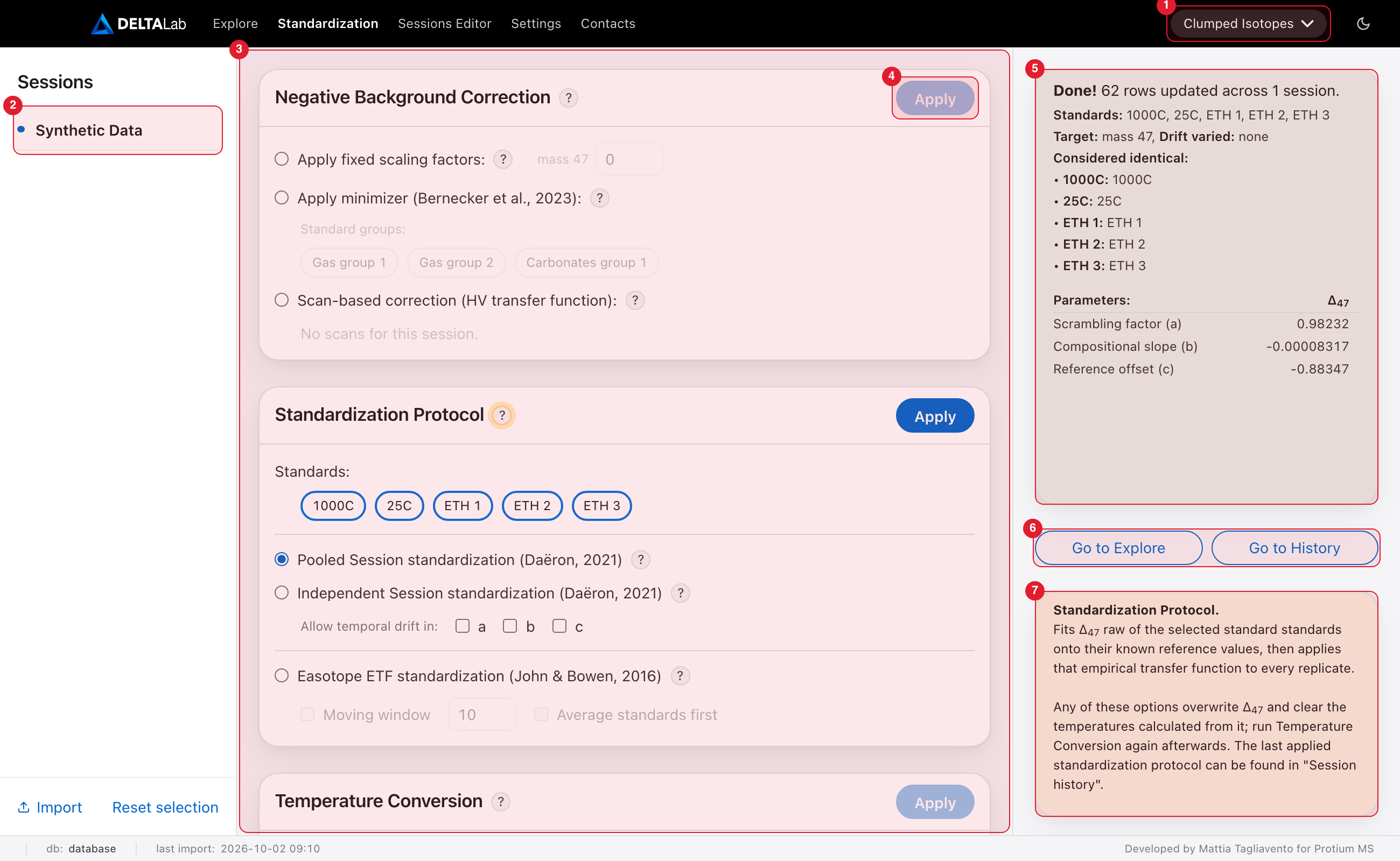
Marked in red: 1 the isotope-system menu, 2 the session list, 3 the cards, 4 a card's Apply button, 5 the result box, 6 Go to Explore and Go to History, 7 the help box.
How the page works
- Choose the isotope system (1). It decides what you calibrate: Δ₄₇ for Clumped Isotopes, Δ₄₇ and/or Δ₄₈ for Dual Clumped.
- Select the session or sessions (2). A card is applied to every selected session. Deactivated sessions are not in this list.
- Work through the cards (3) from top to bottom. The lower cards appear when you scroll the middle column. In each card, choose your options and click Apply (4).
- Read the result box (5) after every Apply.
Good to know:
- Nothing is chosen for you. No method, standard, group or calibration is ticked when you open the page.
- Apply is greyed out until you choose the card's method, protocol or calibration. While a card is working, the button reads Running….
- A green result box means the step was done. A red message means something is missing; it tells you what.
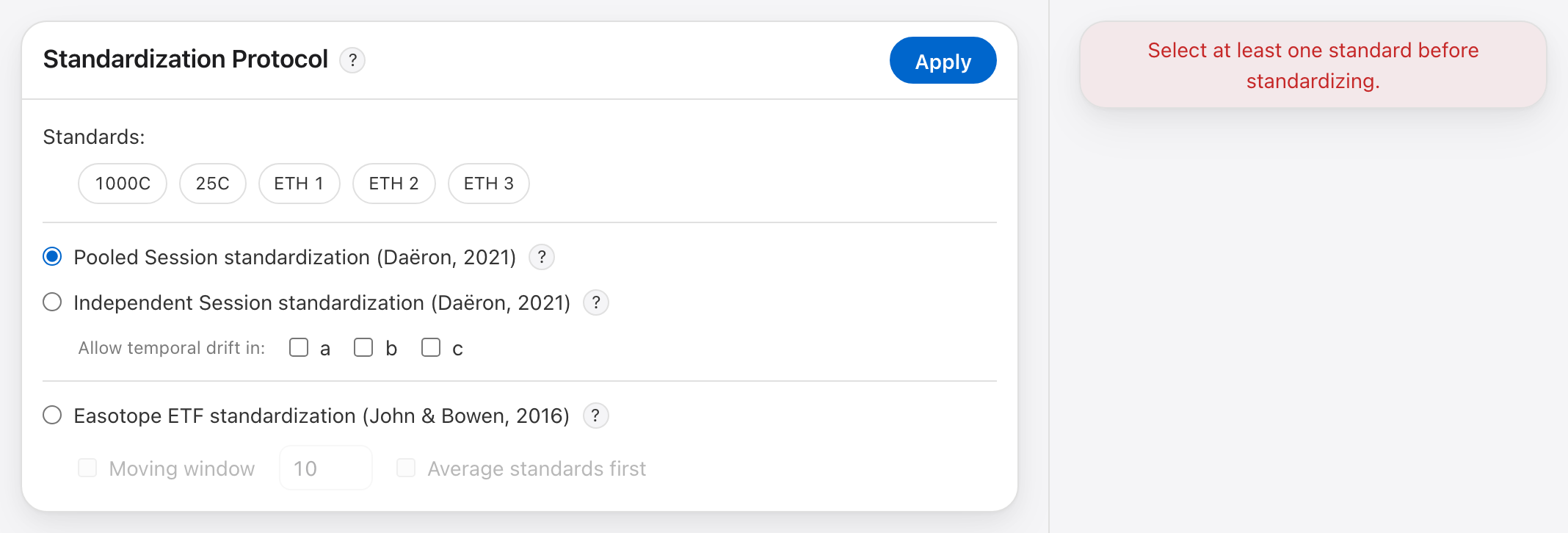
Help ("?") buttons
Every card, and most options, have a ? button. Its text appears in the help box (7).
- Hover over a ? to read its text.
- Click it to keep that text in place while you work. Click another ? to switch, or the same one again to clear the box.
Several help texts name the paper to cite when you use that method.
The result box and the two buttons
After a standardisation the result box (5) shows:
- Done! and how many replicates (rows) were updated, in how many sessions;
- Standards, Target and Drift varied: what you chose, plus ETF option after an Easotope run;
- Considered identical: for each standard, the sample names in your data that were treated as that standard. Check this list. A name you did not expect means a sample is being used as a standard. "No active replicates" means the standard was ticked but has no usable replicate in the selected sessions;
- Parameters: the fitted values, one table per session. Sessions with exactly the same values share one table.
The same record is kept in Session History (chapter 4.3).
The two buttons (6) become active after a Standardization Protocol, Bulk Standardization or δ¹⁸O Acid Fractionation run:
- Go to Explore opens the Explore page (chapter 4) for the sessions you just processed, with the plot already showing corrected values.
- Go to History opens their Session History tab.
What to run again after a change
The cards build on each other. When you run one again, some later results are cleared and others are left as they were.
| You run again | What happens to later results | Then run again |
|---|---|---|
| Negative Background Correction | Δ₄₇ raw is recalculated. Everything after it is cleared: standardised Δ, temperatures, standardised δ¹³C and δ¹⁸O, δ¹⁸O AF | every card you use |
| Standardization Protocol | Standardised Δ is replaced. Temperatures are cleared, because they were calculated from the previous Δ₄₇ | Temperature Conversion |
| Temperature Conversion | Temperatures are replaced | nothing |
| Bulk Standardization | Standardised δ¹³C and δ¹⁸O are replaced. δ¹⁸O AF is cleared | δ¹⁸O Acid Fractionation Correction |
| δ¹⁸O Acid Fractionation Correction | δ¹⁸O AF is replaced | nothing |
Bulk Standardization and the Standardization Protocol do not affect each other.
Excluding or including a replicate also makes a standardisation out of date (red flag, chapter 2). Run the Standardization Protocol again, then Temperature Conversion.
Card: Negative Background Correction
Real data has a negative background on m/z 47. DELTALab removes it from every cycle with the m/z 47.5 half-mass beam:
V47 new = V47 − factor × V47.5
The card needs data that was imported with its raw acquisitions. Choose one of three methods and click Apply.
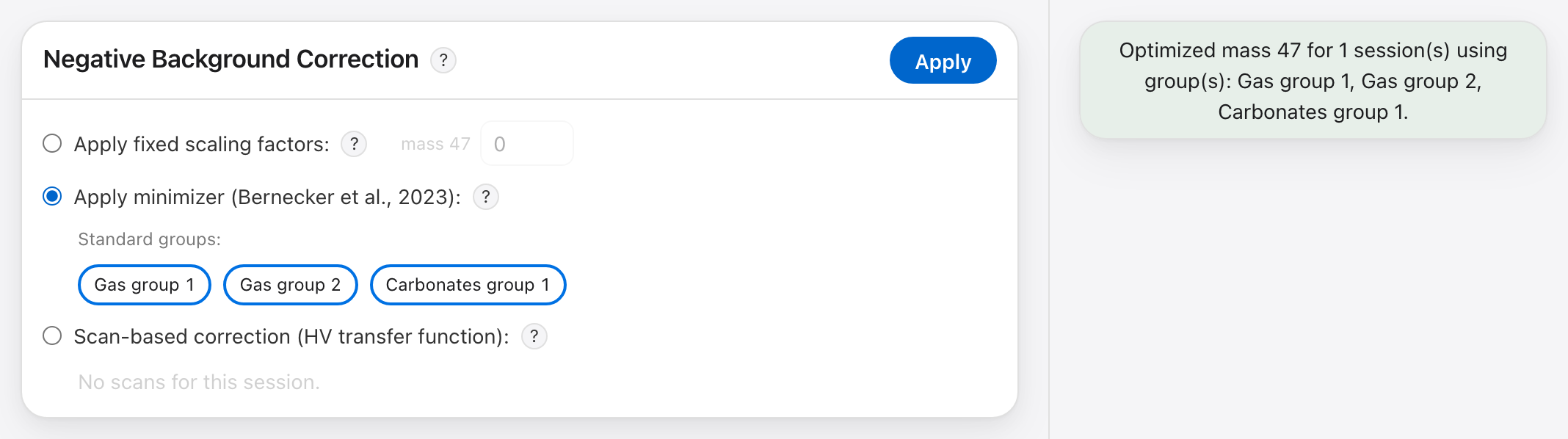
- Apply fixed scaling factors. Type the mass-47 factor. It is applied to every selected session. Type a positive number. This is different from Easotope.
- Apply minimizer (Bernecker et al., 2023). DELTALab finds, for each selected
session, the factor that makes Δ₄₇ raw flattest against δ⁴⁷ within each group
of standards.
- Tick the Standard groups to use.
- Groups come from the Neg. Bkg eval. column of Settings → Reference material (chapter 7). Put standards that were heated or equilibrated at the same temperature in the same group.
- A "Gas" group needs at least one standard; any other group needs at least two. A group with too few is left out.
- The factor that was found is written in Session History (chapter 4.3).
- Scan-based correction (Bernasconi et al., 2013). Uses fitted HV scans instead
of the half-mass beam. It is meant mainly for instruments without an m/z 47.5
cup.
- It works on exactly one session at a time. With no session or several selected, the card says "Select exactly one session to manage its scans."
- The session needs at least one fitted scan set (chapter 6.1). Without one, the card says "No scans for this session."
- Tick the Scan sets to use, then choose how to Combine sets: Nearest, Average or Interpolate. Choose one even if you ticked a single set.
After Apply, Δ₄₇ raw is recalculated and everything after this card is cleared. Run the cards below again.
Card: Standardization Protocol
Fits the Δ₄₇ raw of your standards to their accepted values, then applies that fit to every replicate.
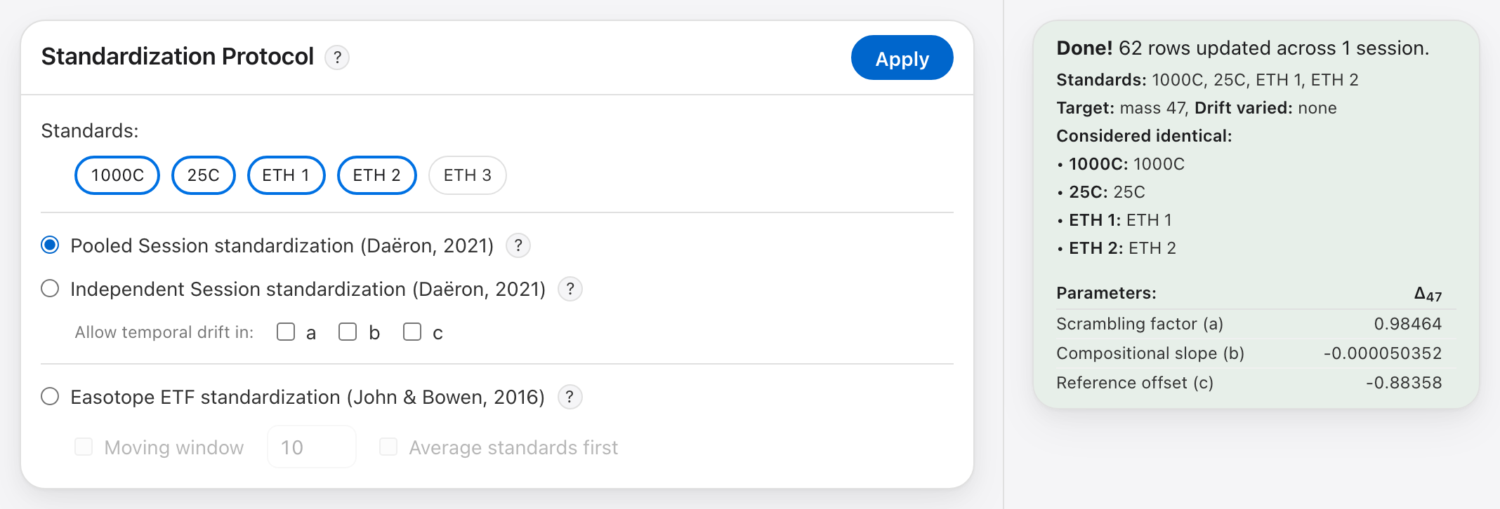
- Tick the Standards. The list shows every reference material from Settings → Reference material (chapter 7), whether or not the selected sessions contain it. This choice has nothing to do with which standards are drawn in the plots.
- Choose the protocol.
- Pooled Session standardization (Daëron, 2021). All selected sessions are fitted together. Each session keeps its own fit, but an unknown measured in several sessions gets one shared Δ₄₇. Use this when your sessions share standards.
- Independent Session standardization (Daëron, 2021). Each session is fitted on its own, from its own standards. An unknown measured in several sessions is reported as the weighted average of its per-session values.
- Easotope ETF standardization (John & Bowen, 2016). Easotope's empirical transfer function. Each session is fitted on its own with a straight line from Δ₄₇ raw to the standards' accepted values, with no δ⁴⁷ term and no drift. Each standard replicate is corrected by the line fitted without itself; every other replicate uses the whole-session line.
- Allow temporal drift in a / b / c (optional, Pooled and Independent only). Tick a coefficient to let it change steadily over time within the fit. a is the scrambling factor, b the compositional slope and c the reference offset, as named in the result box.
- Click Apply.
The Easotope options. Two boxes under the Easotope choice change how its lines are fitted. You can tick one of them or neither.
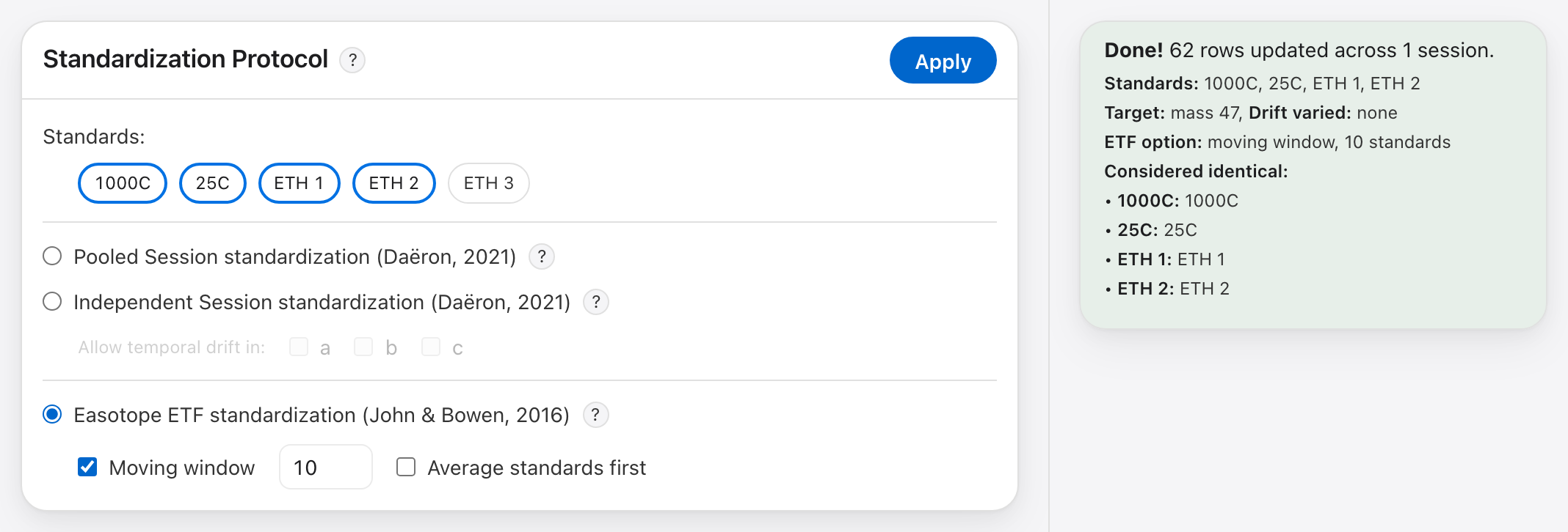
- Moving window: each replicate gets its own line, fitted on the N nearest standard replicates before it and the N after it. Type N in the box; it starts at 10. There is no session line, so the result box has no Parameters table, and replicates you import later stay blank until the next run. If a window holds fewer than two different standards, the run is refused and nothing changes.
- Average standards first: each standard's replicates are averaged, then one line is fitted through those means.
Any protocol replaces the standardised Δ₄₇ of the selected sessions and clears their temperatures, which were calculated from the previous Δ₄₇. T (°C) and T SE show "—" until you run Temperature Conversion again.
Card: Temperature Conversion
Converts the standardised Δ₄₇ of your samples to °C.
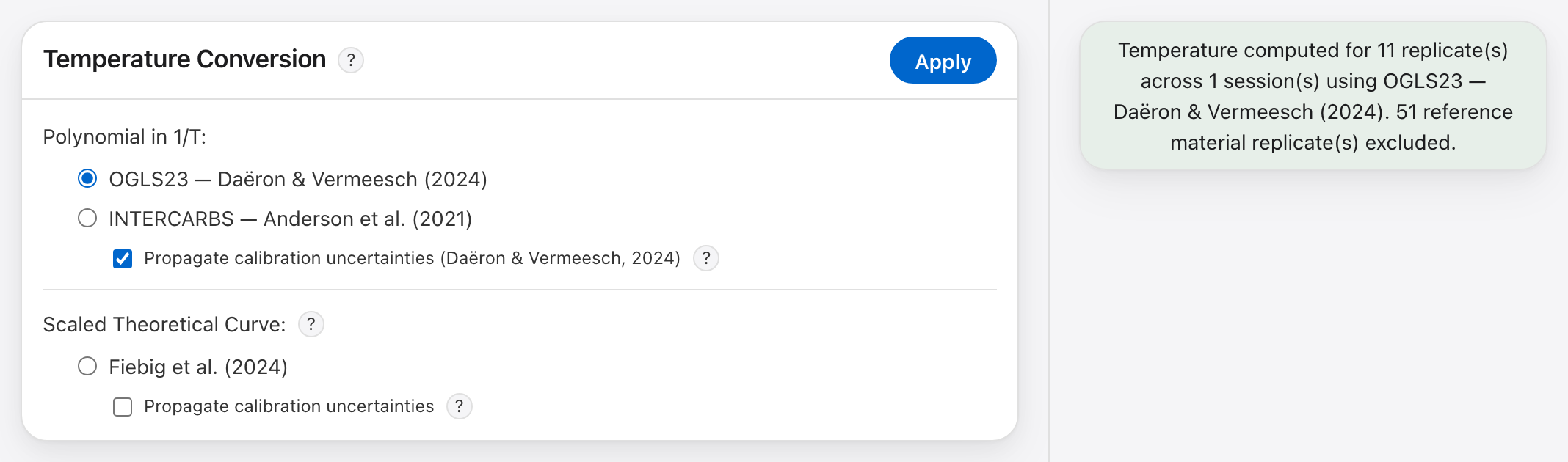
- Pick one calibration. You can only pick one across all groups.
- Tick Propagate calibration uncertainties under that group if you want an uncertainty for each temperature.
- Click Apply.
Good to know:
- Run standardisation first. Raw Δ is never converted. Otherwise a red message tells you to.
- Only Δ₄₇ is converted, even on Dual Clumped. Δ₄₈ is never used for temperature.
- Standards get no temperature. Every sample named in the Reference material table is left out, and the result box says how many replicates that was.
- You manage the list of calibrations in Settings → Temperature calibrations (chapter 7), not here.
- Temperatures outside a calibration's range are still calculated.
The calibrations are grouped by type:
- Polynomial in 1/T:
Δ = a0 + a1·x + a2·x², withx = 1/T. Shipped examples: OGLS23 (Daëron & Vermeesch, 2024) and INTERCARBS (Anderson et al., 2021). - Scaled Theoretical Curve: a fixed theoretical curve with only an offset and a scale fitted. Shipped example: Fiebig et al. (2024).
Propagate calibration uncertainties adds a T SE column. It combines the replicate's Δ uncertainty with the calibration's own uncertainty. Notes at the bottom of the card warn you about any limits:
- Empty error bar: there was no uncertainty information at all. T SE is left empty (not zero).
- Calibration-only / Analytical-only: one of the two uncertainty sources was missing, so T SE is too small.
- Approximate calibration error: the calibration only has a published 1σ for each coefficient, not the full covariance matrix. The error bar comes out about 3–4 times too large.
Card: Bulk Standardization
Standardises δ¹³C and δ¹⁸O. Each session is fitted on its own.
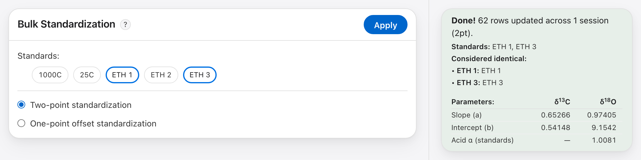
- Tick the Standards. This list is separate from the one in the Standardization Protocol card. Tick standards that have δ¹³C and δ¹⁸O values in the Reference material table.
- Choose the method.
- Two-point standardization: fits a straight line through all the standard replicates.
- One-point offset standardization: shifts every value by the average difference between the standards' measured and accepted values.
- Click Apply.
Both methods use every standard you tick. Raw values are never changed, so you can run this again at any time. A session whose standards have no usable bulk values is skipped, not treated as an error.
How δ¹⁸O is fitted (same as D47crunch): the standards' δ¹⁸O values in the Reference material table are carbonate values. You can enter them on VPDB or on VSMOW (a VPDB value is converted to VSMOW when you save, and the app calculates with the VSMOW value). The instrument measures the CO₂ released by acid digestion, on VSMOW. So each standard's accepted value is first converted to that CO₂ value:
δ¹⁸O CO₂ (VSMOW) = (1000 + δ¹⁸O carbonate (VSMOW)) · α − 1000
α is the calcite acid fractionation factor (Settings → Acid Fractionations) at the session's acid reaction temperature. δ¹⁸O corr is therefore a CO₂ value on VSMOW.
Card: δ¹⁸O Acid Fractionation Correction
Converts standardised δ¹⁸O from the CO₂ produced by acid digestion into the mineral's own δ¹⁸O, using the mineral you pick for each sample and the session's acid reaction temperature.
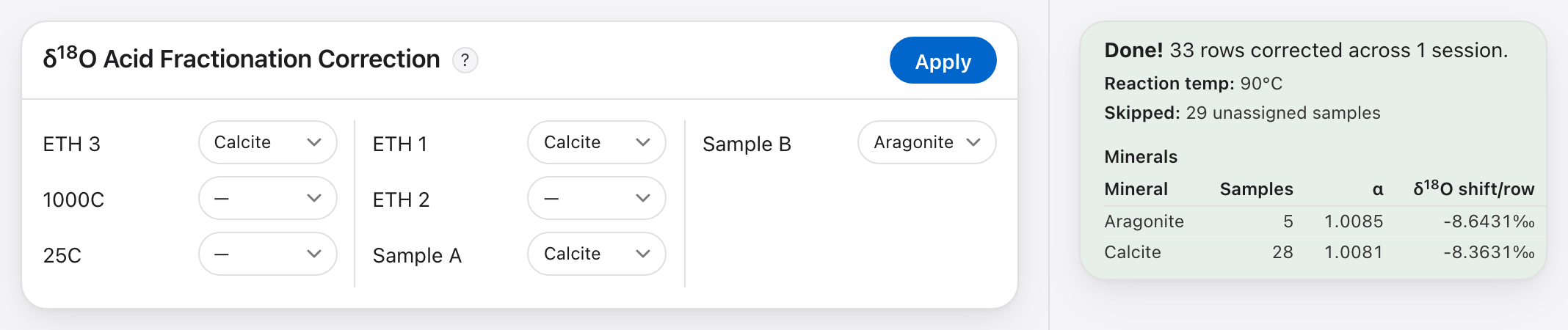
- Run Bulk Standardization first. Until then the list is greyed out and the card says so.
- Pick a mineral next to each sample. Standards are listed first. Leave "—" for anything you do not want corrected.
- Click Apply.
Good to know:
- The result goes into its own δ¹⁸O AF column; δ¹⁸O corr is not changed.
- Your choice of mineral is remembered for each sample name and filled in the next time you open the page.
- The result box shows the reaction temperature used, how many replicates were skipped because they have no mineral, and one line per mineral with its α and its average shift.
Chapter 5.1 covers the whole workflow.
Dual Clumped: what changes
With Dual Clumped chosen in the top bar, the first two cards gain controls for Δ₄₈.
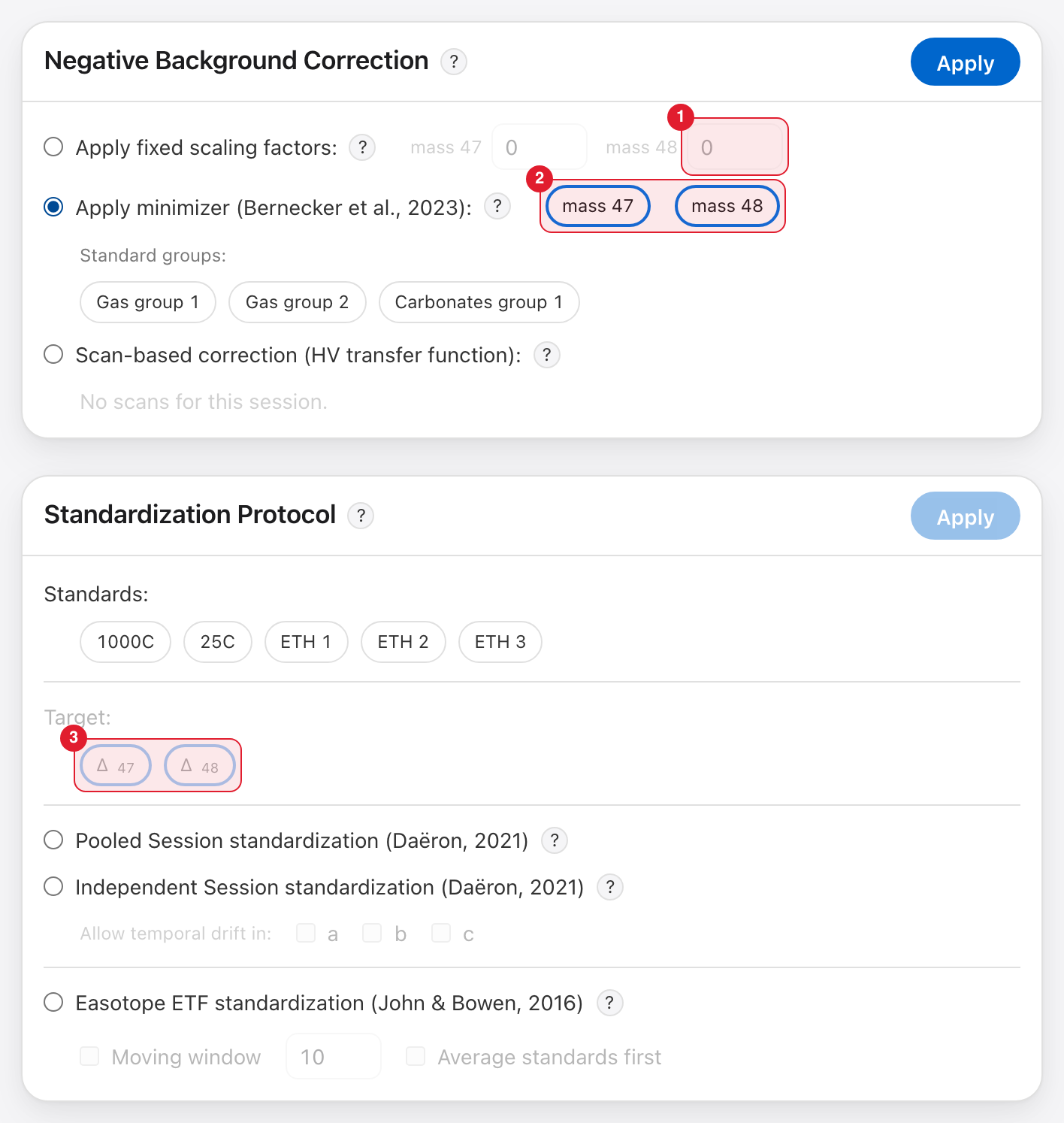
Marked in red: 1 the mass-48 factor, 2 the masses the minimizer works on, 3 the Target.
- Fixed scaling factors (1): a second box for the mass-48 factor.
- Minimizer (2): choose mass 47, mass 48 or both. The two are found separately, from the same standard groups.
- Target (3): standardise Δ₄₇, Δ₄₈ or both, with any of the three protocols. Both are ticked at the start. The result box then shows a column of parameters for each. A run with only Δ₄₈ ticked leaves Δ₄₇ and the temperatures as they were.
- Scan-based correction only lists scan sets that have a fit for mass 48 as well as mass 47.
Temperature Conversion, Bulk Standardization and the δ¹⁸O acid correction work the same in both systems.
5.1 The δ¹⁸O acid fractionation correction
Carbonates are measured as the CO₂ released when they react with phosphoric acid. That CO₂ is richer in ¹⁸O than the mineral it came from, by an amount that depends on the mineral and on the reaction temperature. The δ¹⁸O Acid Fractionation Correction removes that offset and gives you the δ¹⁸O of the mineral itself.
The result goes into its own column, δ¹⁸O AF. Nothing else changes: δ¹⁸O corr, δ¹³C, Δ₄₇, Δ₄₈ and temperatures stay exactly as they were.
The equation
For each replicate DELTALab computes the acid fractionation factor α of the sample's mineral at its session's reaction temperature:
1000 ln α = a·10⁶/T² + b·10³/T + c
Tis the session's acid reaction temperature in kelvin (°C + 273.15).a,bandcare the mineral's constants from Settings → Acid Fractionations.
Then it computes the mineral value from the standardised one:
δ¹⁸O AF = (δ¹⁸O corr + 1000) / α − 1000
At 90 °C, calcite gives α ≈ 1.00813: a δ¹⁸O corr of 30.00 ‰ gives a δ¹⁸O AF of about 21.70 ‰.
Before you start: standard δ¹⁸O values are carbonate values
The correction treats δ¹⁸O corr as the δ¹⁸O of the CO₂. Bulk Standardization makes it one: it converts each standard's accepted carbonate value into the CO₂ it releases, using calcite's α at the session's reaction temperature (chapter 5).
The δ¹⁸O values shipped for ETH-1 to ETH-3 in the Standards table are carbonate values on VPDB, as published. If you add your own bulk standards (Settings → Reference material), enter their δ¹⁸O as carbonate values on VPDB too. A CO₂ value there would be shifted by α a second time.
Because the standards go through the same α, a standard whose mineral is set to calcite gets back its own accepted value in δ¹⁸O AF.
Overview of the workflow
- Settings → Acid Fractionations: check that every mineral you need is in the list, with the right constants and reference. Done once, not per session.
- Sessions Editor: set each session's acid reaction temperature.
- Standardization page: run Bulk Standardization.
- Standardization page: pick a mineral for each sample on the δ¹⁸O Acid Fractionation Correction card and click Apply.
- Read the result box, then check the values: pick δ¹⁸O AF in the Replicates list's δ¹⁸O menu, or look at the Summary table's δ¹⁸O AF column.
Steps 1 and 2 can be done in any order, but both must be done before step 4.
Step 1: Check the minerals in Settings
Open Settings and find the Acid Fractionations table. Each row is one mineral with its reference and its three constants. DELTALab ships with:
| Mineral | a | b | c | Reference |
|---|---|---|---|---|
| Calcite | 0 | 3.59 | −1.79 | Kim, Mucci & Taylor (2007) |
| Aragonite | 0 | 3.39 | −0.83 | Kim, Mucci & Taylor (2007) |
| Magnesite | 0.6845 | 0 | 4.22 | Das Sharma, Patil & Gopalan (2002) |
These are ordinary entries: you can edit or delete them like any other.
To add a mineral:
- Click Add next to the table title.
- Type the Mineral name, for example
Dolomite. - Type the Reference: the paper the equation comes from. It is required.
- Type
a,bandc(see the next section). Use0for a term the paper's equation doesn't have; a blank field is refused. - Click Save.
To edit or delete a mineral: click the pencil icon on its row. The window has the same fields, plus Delete mineral at the bottom left.
A reference shown as Missing in red belongs to a mineral carried over from an older version of DELTALab. Edit it and type the source paper.
Editing a mineral does not change values already corrected with it. The constants are read when you click Apply. Click Apply again to bring existing values in line.
Turning a published equation into a, b and c
Papers give the acid fractionation factor in a few different ways. Rewrite the
paper's equation so that it reads 1000 ln α = …, then read off:
a: the number in front of10⁶/T²;b: the number in front of10³/T;c: the number that stands on its own.
Example 1: Das Sharma, Patil & Gopalan (2002), magnesite. The paper's form is
α = exp((4.22 + 6.845·10⁵/T²) / 1000)
- Take the natural log of both sides:
ln α = (4.22 + 6.845·10⁵/T²) / 1000. - Multiply both sides by 1000:
1000 ln α = 4.22 + 6.845·10⁵/T². - Write
6.845·10⁵/T²as0.6845 · 10⁶/T². - Read off
a = 0.6845,b = 0,c = 4.22.
Example 2: Kim, Mucci & Taylor (2007), calcite. The paper gives
1000 ln α = 3.59 · (10³/T) − 1.79, which already has the right form:
a = 0, b = 3.59, c = −1.79.
The same equation is sometimes written as α = exp(3.59/T − 1.79·10⁻³). Multiply
the exponent by 1000 and you get 3.59·10³/T − 1.79, so c is still −1.79.
Watch the factor of 1000. It is the most common way to get a constant wrong.
cis−1.79, not−0.00179, andbis3.59, not3590. A quick check: at 90 °C a carbonate's α should lie roughly between 1.007 and 1.011. The α column in the result box (step 4) shows the value actually used.
Step 2: Set each session's acid reaction temperature
Each session stores the temperature of its acid bath.
- Open Sessions Editor in the top bar and click the session on the left.
- Click Edit. The Edit session window opens.
- Under Acid reaction temperature, type the temperature in °C.
- Click Save.
Good to know:
- If you never set a temperature, 90 °C is used. The box is then empty.
- Saving a temperature recalculates nothing. It takes effect the next time you run Bulk Standardization (the standards' α) and click Apply on the correction card (the samples' α). Re-run both after changing it.
- Different sessions can have different temperatures. When you correct several sessions at once, each replicate uses its own session's temperature.
Step 3: Run Bulk Standardization
The correction works on standardised δ¹⁸O (δ¹⁸O corr), never on the raw value. Run the Bulk Standardization card for your sessions first (chapter 5).
Until at least one selected session has been bulk standardised, the correction card is greyed out and says so.
Step 4: Assign minerals and apply
On the Standardization page, select your sessions in the list on the left, then scroll to the δ¹⁸O Acid Fractionation Correction card (below Bulk Standardization).
The card lists every sample in the selected sessions, in three columns. Standards are listed first, then your other samples. Next to each sample is a menu of the minerals from Settings.
- Pick a mineral for each sample you want to correct.
- Leave a sample on — to skip it. It gets no δ¹⁸O AF value (or keeps the one from an earlier Apply).
- Standards can be corrected too; they are listed first only to keep them together.
- Click Apply at the top right of the card.
Apply stays disabled until at least one sample has a mineral.
DELTALab remembers your choices. When you click Apply, every sample's mineral is saved and filled in the next time you open the card, for any session containing that sample. To change a sample's mineral, pick a different one. Choosing — only clears it for this visit; the saved mineral comes back next time.
Reading the result
After Apply, a result box opens under the page header:
- Done! N rows corrected across M sessions.
- Reaction temp: the temperature used. One value if every session shared it,
otherwise one per session, for example
Run A: 90°C, Run B: 70°C. - Skipped (only if something was skipped):
- unassigned samples: replicates whose sample had no mineral;
- samples not yet bulk standardized: replicates with no δ¹⁸O corr yet, usually from a session you haven't bulk standardised. They get no δ¹⁸O AF.
- Minerals: a table with one row per mineral used in this run:
| Column | Meaning |
|---|---|
| Mineral | The mineral's name |
| Samples | How many replicates were corrected with it |
| α | The fractionation factor used. Two values separated by / mean the mineral was applied at two different session temperatures |
| δ¹⁸O shift | The average of δ¹⁸O AF − δ¹⁸O corr per replicate, in ‰. It is negative: the mineral is lighter than its CO₂ |
Go to Explore and Go to History take you to the corrected values and to the log entry.
Where the corrected values appear
- Replicates (chapter 4): choose δ¹⁸O AF in the menu of the δ¹⁸O column header. Hover over a value to see the δ¹⁸O corr and raw values behind it.
- Summary table: a δ¹⁸O AF column appears right after δ¹⁸O as soon as any replicate in view has a corrected value. It is the sample mean; a sample never corrected shows "—".
- Plots: the δ¹⁸O plot on the δ¹⁸O tab shows δ¹⁸O corr, not δ¹⁸O AF.
- Export report: the replicates table has a
d18O_AFcolumn, and the summary hasd18O_AF_meanandd18O_AF_std. They are blank for samples never corrected. - Session History: each session gets a δ¹⁸O AFF entry with the minerals, the reaction temperature and the number of replicates corrected.
The correction never changes the raw δ¹⁸O (chapter 1).
Changing or redoing a correction
Apply always starts from δ¹⁸O corr, never from an earlier δ¹⁸O AF. So you can click it as often as you like: the same minerals and temperatures always give the same result.
- After changing a sample's mineral, a mineral's constants or a session's temperature: click Apply again. The new values replace the old ones.
- After re-running Bulk Standardization: δ¹⁸O AF is cleared for the replicates it standardised, because it was computed from the old δ¹⁸O corr. Your minerals are still filled in on the card; click Apply again.
- Importing new replicates or reprocessing a session also leaves those replicates without a δ¹⁸O AF until you apply again.
Sessions corrected before this version. Earlier versions wrote the correction over δ¹⁸O corr itself. For a session corrected that way, re-run Bulk Standardization once to restore δ¹⁸O corr, then click Apply.
Quick checklist
- [ ] The minerals you need are in Settings → Acid Fractionations, each with a reference.
- [ ] Your bulk standards' δ¹⁸O values are carbonate values on VPDB.
- [ ] Every session has the right acid reaction temperature (default 90 °C).
- [ ] Bulk Standardization has been run.
- [ ] Every sample to correct has a mineral on the card.
- [ ] Apply clicked since the last Bulk Standardization.
- [ ] The α values in the result box look sensible (≈ 1.007–1.011 at 90 °C).
6. The Sessions Editor
The Sessions Editor is where you fix how your data is organised: a session's name, instrument and reference gas, a mislabelled sample, a replicate that landed in the wrong session, a session that should be two. It is also where you set a session aside, or delete data.
It is the safe place for these changes. Every edit here also updates the raw acquisitions and marks the standardisation as out of date when it should be.
Open Sessions Editor in the top bar and click a session on the left. You work on one session at a time.
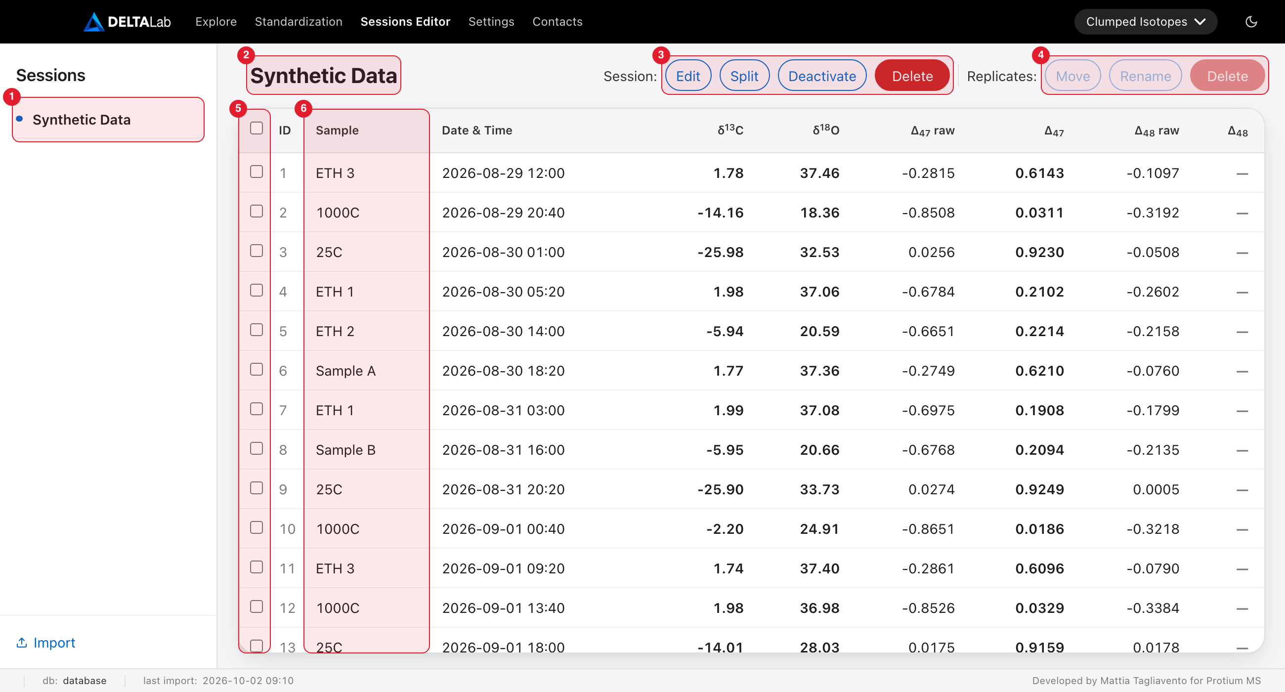
Marked in red: 1 the session list, 2 the session name, 3 the session buttons, 4 the replicate buttons, 5 the tick boxes, 6 the sample names.
The page at a glance
- The session list (1) works like the one on the Explore page, but you pick one session only.
- The session name (2) is pale grey when the session is deactivated.
- The session buttons (3) act on the whole session: Edit opens the Edit session window, then Split, Merge, Deactivate and Delete.
- The replicate buttons (4) act on the replicates you ticked: Move, Rename and Delete.
- The tick boxes (5) choose replicates. The box in the header ticks or clears all of them.
- A sample name (6) opens that replicate's acquisitions window, the same one as in the Replicates (chapter 4.1).
The table shows one row per replicate. Δ₄₇ and Δ₄₈ are the standardised values; they show "—" until the session is standardised. δ¹³C and δ¹⁸O turn bold once they are standardised; hover one to see its raw value.
One rule decides which buttons work:
- Nothing ticked: the session buttons work. The replicate buttons are greyed out.
- One or more replicates ticked: the replicate buttons work. The session buttons are greyed out until you clear the ticks.
After each change, a line under the buttons tells you what was done.
What each action does to your results
| Action | Values recalculated | Run standardisation again | Safety backup first |
|---|---|---|---|
| Rename the session | no | no | no |
| Change the mass spectrometer | no | no | no |
| Change the reference gas | yes | yes | no |
| Change the acid reaction temperature | no | only Bulk Standardization and the δ¹⁸O acid correction | no |
| Split | no (the numbers stay the same) | yes, every part | yes |
| Merge | yes, the replicates merged in | yes, the merged session | yes |
| Deactivate, Activate | no | no | no |
| Delete the session | — | — | yes |
| Move | no | yes, both sessions | no |
| Rename (sample name) | no | yes | yes |
| Delete replicates | no | yes | yes |
A new reference gas or a split clears the session's standardised values and temperatures. Δ₄₇ shows "—" until you run standardisation again (chapter 5). The session gets no red flag (chapter 2), because nothing out of date is left on screen.
Move, Rename and Delete replicates leave every value where it is and give the session a red flag. The standardised values on screen are then out of date until you run standardisation again.
Safety backups are restored with Settings → Restore backup (chapter 8).
Every action except deleting a session is written to Session History (chapter 4.3). Deleting a session deletes its history too.
Editing a session: name, instrument, reference gas, acid temperature
Click Edit.
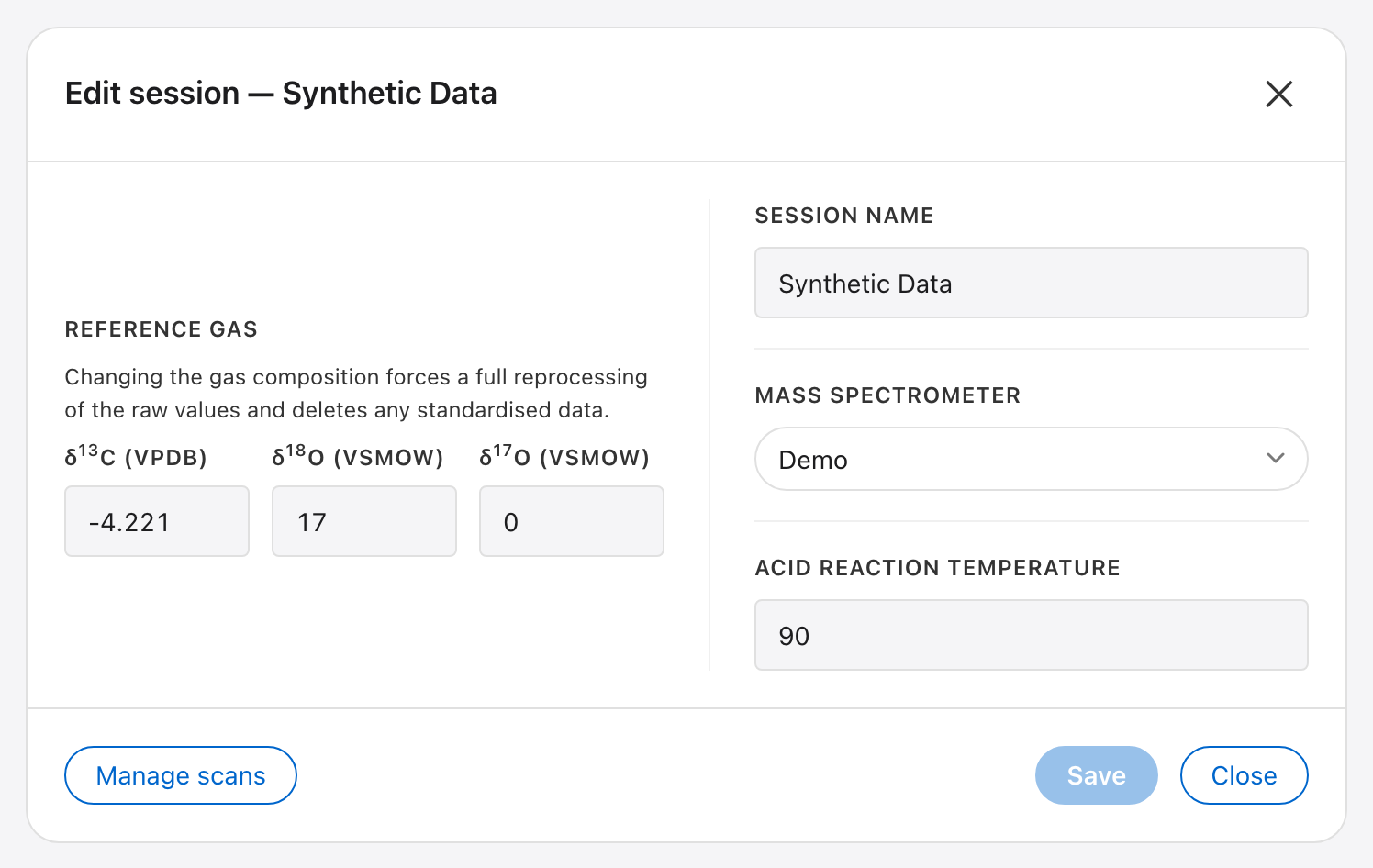
Change what you need, then click Save. It saves everything you changed, and it stays greyed out until you have changed something. Close only closes the window and forgets anything you did not save.
- Session name. Only the name changes; nothing is recalculated. A blank name, or a name another session already uses, is refused.
- Mass spectrometer. If your lab has several instruments, the session moves to that instrument's group in the session list. Nothing is recalculated, and the session keeps its own reference gas and acid temperature. New instruments are added in Settings (chapter 7) or in the import window.
- Reference gas. δ¹³C (VPDB) and δ¹⁸O (VSMOW) of the reference gas. While you have changed one of them, the button reads Save & reprocess. The session's values are recalculated with the new gas and its standardised values are cleared, so run standardisation again (chapter 5). δ¹⁷O is not used for carbonate or CO₂ data.
- Acid reaction temperature. The temperature of the acid bath in °C, used by the δ¹⁸O acid fractionation correction (chapter 5.1). Nothing is recalculated at that moment. If the session has no temperature, the box is empty and 90 °C is used.
Manage scans, at the bottom left, opens the scan sets of this session (chapter 6.1).
A new session gets its reference gas and acid temperature from its mass spectrometer when you import it (chapter 3). Use this window when one session needs different values, for example after a new reference gas tank.
Deactivating a session
Deactivate sets a session aside without deleting anything, for example a failed run you want to keep.
- It turns pale grey in the session list and stays visible on the Explore page, where you can still look at it.
- It is left out of the Standardization page, of Export report and of the Existing session list in the import window.
- Nothing is deleted or recalculated.
While a session is deactivated the button is blue and reads Activate. Click it to bring the session back. Both changes are written to Session History (chapter 4.3).
Fixing a mislabelled sample
A replicate has the wrong sample name, for example a typo or the wrong standard.
- Tick the mislabelled replicate, or several that need the same name.
- Click Rename.
- Type the correct name, or pick one of the session's sample names from the list under the box.
- Click Rename in the window.
- Run standardisation again.
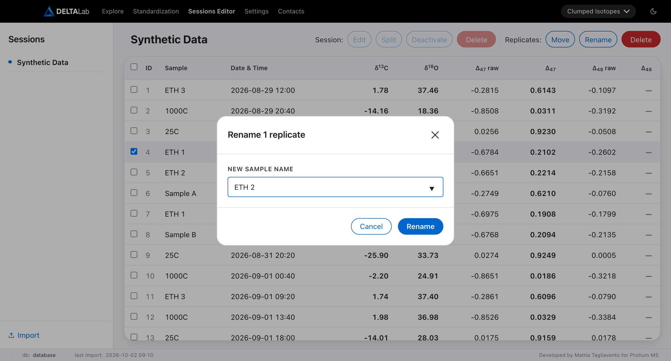
What happens:
- DELTALab takes a safety backup and renames the replicate's raw acquisitions.
- The replicate's values stay as they were, and the session gets a red flag.
- Exclusions are kept.
- A name that matches a reference material makes the replicate a standard, so it can be used as a standard. A name that matches none makes it a sample.
- A replicate stays a replicate of its own, even when its new name is the same as the replicate just before or after it.
Don't fix a sample name by editing the database tables directly. That leaves the raw acquisitions unchanged, so the next recalculation brings the wrong name back. It also skips Session History and does not mark the standardisation as out of date.
Moving replicates to another session
Use Move when replicates were imported into the wrong session.
- Tick the replicates.
- Click Move.
- Pick the Destination session.
- Click Move in the window.
- Run standardisation again for both sessions.
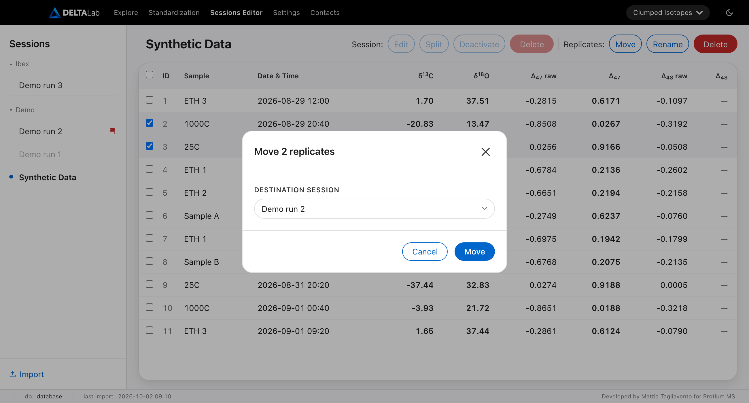
Good to know:
- The destination must already exist. To put replicates into a new session, use Split instead.
- Moved replicates keep their values and their exclusions. Nothing is recalculated until you standardise.
- Both sessions get a red flag.
- Moved replicates keep the background correction they had. If the two sessions use different corrections, run the Negative Background Correction for the destination session (chapter 5).
- Files and notes attached to a replicate move with it.
- A session you move every replicate out of disappears from the list.
Splitting a session
Sometimes one session covers more than one real run: an overnight gap, an instrument re-tune, a new reference gas. Split turns it into two or three sessions. No measured number changes, only which session each replicate belongs to.
Split needs at least two replicates in the session.
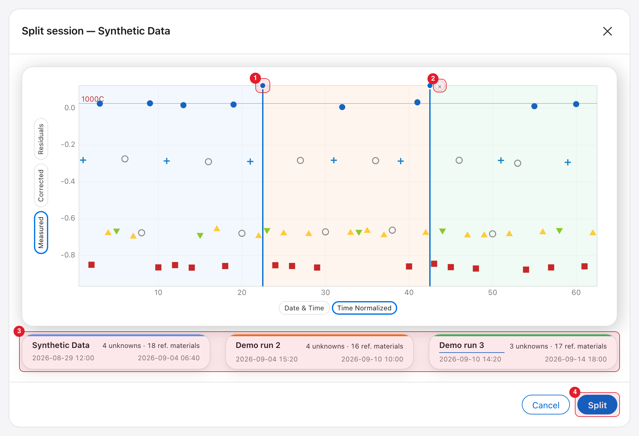
Marked in red: 1 a cut and its handle, 2 the × that removes a cut, 3 the part cards, 4 the Split button.
- Click Split. The window shows the session's plot.
- Click the plot where a new session should start. A line appears (1). You can place up to two cuts, which gives three sessions. A cut always falls between two replicates.
- Adjust the cuts:
- drag the handle on top of a line to move the cut;
- hover the handle and click the × (2) to remove the cut.
- Check the part cards (3). Each part has its own colour, on the plot and on its card. A card shows the part's name, its number of unknowns and reference materials, and its first and last date.
- Name the new parts: click a name to edit it. The first part keeps the original session's name.
- Click Split (4) at the bottom of the window. DELTALab takes a safety backup first.
Good to know:
- The buttons on the plot work as on the Explore page (chapter 4). Date & Time helps you find a gap in time; Time Normalized spaces the replicates evenly, which makes a cut easier to place.
- The plot follows the isotope system chosen in the top bar.
- If a name is blank or already in use, the card says so in red and the Split button stays greyed out until you fix it.
- A dotted line under the reference-material count means the part has fewer than three different standards. On its own it may not have enough standards for a fit. You can still split, and standardise the part together with other sessions.
- To rename the first part, use Edit after the split.
What the new sessions keep:
- every replicate's raw values, exactly as they were;
- exclusions;
- the background correction, with its own copy of any scan set the session used. Editing one part's scan set later does not change the others;
- the reference gas, the mass spectrometer and the acid reaction temperature.
What they do not keep: the standardisation. Every part, including the one that kept the original name, shows "—" for Δ₄₇ and must be standardised again. The old fit described the whole session, not its parts.
The background correction is copied, not fitted again. If a part should have its own, for example because it now covers a single reference gas, run the Negative Background Correction for that session (chapter 5).
Merging sessions
Merge is Split the other way round. It joins other sessions into the one that is open, for example a run that was imported in two parts. The open session is the target: it keeps its name and its settings. The sessions you tick are the sources: their replicates move into the target and the source sessions disappear.
- Open the target session and click Merge. The window shows the plot of the session and a list called Add sessions.
- Tick the sessions to add. Click anywhere on a row. The plot draws the replicates of every ticked session and, when the sessions do not overlap in time, shades each one in the colour of its card.
- Check the cards under the list: one for the target, one for each ticked session, and a Result card with the totals.
- Click Merge. DELTALab takes a safety backup first.
After the merge a line under the buttons tells you what was done, and the history of the target shows a Merge entry.
Good to know:
- Only sessions that fit are offered. A session must come from the same instrument, use the same reference gas and belong to the same isotope system as the target. A line under the list says how many other sessions cannot be merged; hover it to see why. If a reference gas has a typo, fix it with Edit first.
- The target keeps its settings. Every replicate that moves in is recalculated under the target's reference gas and background correction, exactly as with Move. A source that used another background correction gets the target's. If needed, run the Negative Background Correction again (chapter 5).
- The sources disappear. Their attachments and scan sets come along. Their history stays in the database.
- Run standardisation again for the merged session. Its old fit does not cover the new replicates.
- If the sessions overlap in time, the plot is not shaded by session and a note says so.
Deleting replicates or a session
Both are permanent. DELTALab takes a safety backup first; restoring that backup is the only way back (chapter 8).
To leave a replicate out of the calculations but keep it, exclude it instead (chapter 4.1). To set a whole session aside, use Deactivate.
Delete replicates
- Tick the replicates.
- Click Delete after "Replicates:". The window lists their sample names.
- Type
DELETEin the box. - Click Delete permanently.
The replicates and their raw acquisitions are removed. The other replicates keep their values and the session gets a red flag, so run standardisation again. Replicates on either side of a deleted one stay separate, even if they have the same sample name. If you delete every replicate, the session disappears from the list.
Delete the session
- Clear any ticks and click Delete after "Session:".
- Type the session's name exactly as shown.
- Click Delete permanently.
This removes the session's replicates and raw acquisitions, its scan sets, its attached files and its Session History.
6.1 Scans and the pressure-baseline correction
You only need this chapter if you use the scan-based method on the Negative Background card. It uses scan sets: 1 to 6 HV scans grouped together. DELTALab fits the m/z 47 (and 48) background against the m/z 44 intensity across them (the pressure-baseline method of Bernasconi et al., 2013).
Where: Sessions Editor → click a session → Edit → Manage scans, at the bottom left of the window. A scan set belongs to one session. The session already knows its instrument, so you are not asked for one.
Steps:
- Create a set. Under New set (bottom left), click Choose files and pick
1–6
.scnfiles. Type a name if you like, then click Create set. - Open the set. Click it in the list on the left. Use the m/z 44 to m/z 49 buttons to see each cup's raw trace.
-
Set the windows by dragging on the plot. There are no number fields.
- On-peak window (mass 44): drag across the flat top of the m/z 44 peak. Auto peak makes a first guess; move it to the flat middle.
- Background windows (mass 47, and mass 48 for Dual Clumped): one or two windows per mass, in the flat baseline on either side of the peak. Auto windows makes a first guess, but always check it. Choosing the baseline is a scientific judgement. Clear left and Clear right remove a window.
- Masses 45, 46 and 49 are for viewing only.
- To zoom in on an area of this plot, hold Option (Alt on Windows) and drag a rectangle over it.
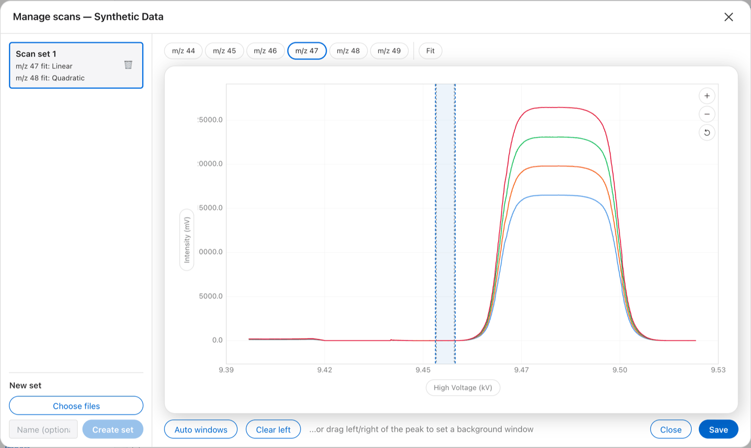
The m/z 47 view. The shaded band left of the peak is a background window; drag on the plot to move it or add one on the right.
-
Check the fit. Click Fit (next to the mass buttons) to see background against m/z 44 intensity, with the fitted line. Choose Linear or Quadratic for each mass; the plot updates as you choose. Click Save.
- Use it. On the Standardization page, pick the set(s) on the Negative Background card and click Apply.
If you change a fit later, it is used the next time the session is processed. You cannot delete a scan set while a session still uses it.
7. Settings
Settings holds the values your whole lab shares: the reference materials, your instruments, the physical constants, the temperature calibrations and the acid fractionation minerals. It also holds a few display choices and the functions for your databases and backups.
The page is one long list of sections. From top to bottom:
- Reference material
- Mass spectrometers
- Computational variables and Temperature calibrations, side by side
- δ¹⁸O Acid Fractionations
- Display preferences and Additional Functions, side by side
Changing a value here recalculates nothing. A changed value is used the next time you run the step that needs it:
| You change | It is used by | From when |
|---|---|---|
| A standard's accepted values | Standardization Protocol, Bulk Standardization | the next time you run them |
| A standard's group (Neg. Bkg eval.) | the background minimizer | the next time you run it |
| A standard's Show in plots boxes | the plots and tables of the Explore page | at once |
| A temperature calibration | Temperature Conversion | the next time you run it |
| A mineral's constants | δ¹⁸O Acid Fractionation Correction; calcite is also used by Bulk Standardization | the next time you run them |
| A computational variable | the calculation of the raw values | the next time a session is imported or recalculated |
| A mass spectrometer's values | new sessions | sessions you import from now on |
The processing steps are described in chapter 5.
Reference material
The table of your standards and their accepted values.
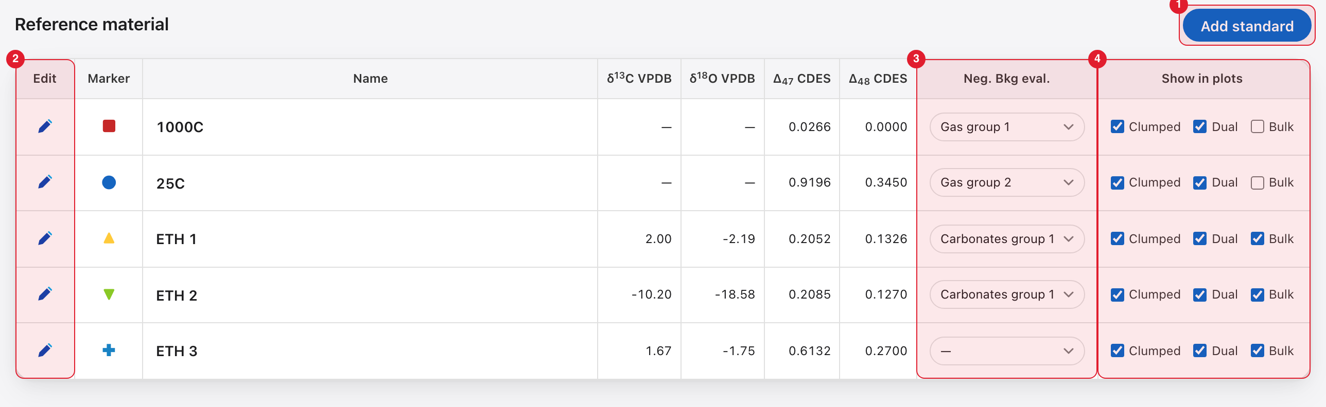
Marked in red: 1 Add standard, 2 the pencils, 3 the Neg. Bkg eval. menus, 4 the Show in plots boxes.
- Δ₄₇ CDES and Δ₄₈ CDES are the accepted values the Standardization Protocol fits to.
- δ¹³C VPDB and δ¹⁸O VPDB are the accepted values Bulk Standardization fits to. δ¹⁸O is the carbonate value (chapter 5.1).
- A value shown as "—" is empty: the standard has no accepted value for that step. The equilibrated gases, for example, have no δ¹³C or δ¹⁸O.
Neg. Bkg eval. (3) puts the standard in a group: Gas group 1–4, Carbonates group 1–4, or "—" for none. The background minimizer assumes all standards in a group share the same true Δ₄₇. The choice is saved as soon as you make it.
Show in plots (4) has one box each for Clumped, Dual and Bulk. The boxes are saved as soon as you tick them.
- A ticked box means the standard is drawn, and counted as a standard, on that system's Explore page (chapter 4). Bulk is for the δ¹³C and δ¹⁸O tabs of both systems.
- The boxes do not decide which standards are used in a fit. You choose the standards on the Standardization page.
To edit a standard, click its pencil (2).
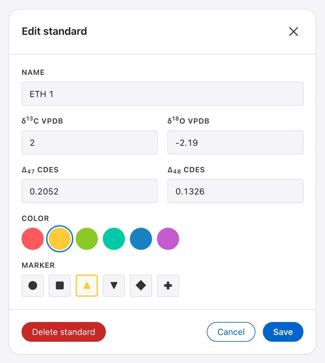
- Change the name, the four values, the Color and the Marker shape, then click Save. Leave a value empty if the standard has none.
- Delete standard removes it after you confirm.
To add a standard, click Add standard (1). The same window opens, empty. Type a name, fill in the values you have and click Save. Nothing is added until you save, so Cancel leaves the table as it was. A name is required, and a name another standard already uses is refused. The new standard's Show in plots boxes start empty, so tick the systems you use it in.
How a sample name is matched to a standard. A replicate counts as a standard when its sample name is the standard's name:
- capitals do not matter;
- a space in the standard's name may also be a hyphen, an underscore or nothing:
"ETH 1" matches
ETH 1,ETH-1,ETH_1andeth1; - a short replicate label may follow, after a space, hyphen or underscore: a
one- or two-digit number, also written with
run,rep,ror#, or a single letter. "ETH 1" matchesETH 1 rep2,ETH-1 #3andETH 1 a.
Anything else is a sample: ETH 10, ETH 1 dup and My ETH 1 do not match
"ETH 1". Name your standards the way they are written in your data. After a
standardisation, the result box lists the names that were matched
(chapter 5).
Mass spectrometers
Your lab's instruments. They appear in the import window and group the session list. Each instrument has its own δ¹³C ref, δ¹⁸O ref and Acid temp, because each one has its own reference gas tank and acid bath. There is no lab-wide default: every session belongs to an instrument and takes its values from it. The first instrument was created when you first started DELTALab.

- Add opens a window with the name and the values (the temperature starts at 90 and the others at 0). All of them are required. δ¹⁷O ref is not used for carbonate or CO₂ data, so leave it at 0.
- A pencil edits the name and the values. A value cannot be left empty.
- Changed values apply to sessions you import from now on. A session copies the values when it is created and keeps them. To change a session that already exists, use the Sessions Editor (chapter 6).
- A changed name is changed for the instrument's sessions too.
- Delete mass spec, in the Edit window, is refused while any session belongs to the instrument. Move those sessions to another instrument in the Sessions Editor first.
Computational variables
The four physical constants used to calculate the raw values: ¹⁷O/¹⁶O (VSMOW), ¹⁸O/¹⁶O (VSMOW), ¹³C/¹²C (VPDB) and λ. They apply to every session.
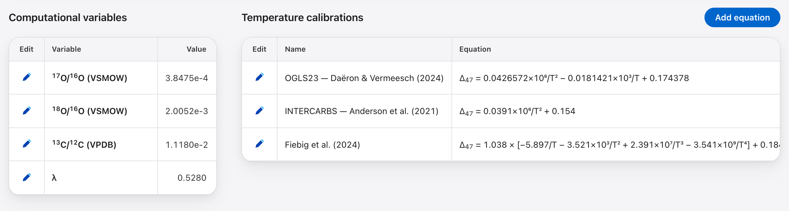
Click a pencil, type the new value and click Save. Saving recalculates nothing. The new value is used the next time a session is imported or recalculated, so sessions processed before and after the change no longer use the same constants. Change these only if you know why.
Temperature calibrations
The list of Δ→T equations offered by the Temperature Conversion card, beside the computational variables. The Equation column shows each one as DELTALab will use it.
A new install includes three Δ₄₇ calibrations:
- OGLS23 (Daëron & Vermeesch, 2024)
- INTERCARBS (Anderson et al., 2021)
- Fiebig et al. (2024)
They are only a starting set. You can change or delete them. Only Restore Default Settings brings the shipped ones back.
Click Add equation to add one, or a pencil to edit one. Nothing is stored until you click Save. The window asks for a Name and a Model.
Model: Polynomial in 1/T
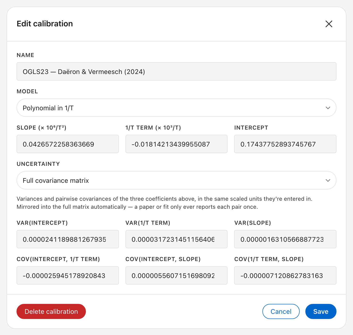
- Type the Slope, the 1/T term and the Intercept. The slope is the
number in front of 10⁶/T² and the 1/T term is the number in front of 10³/T. For
Δ₄₇ = 0.0391×10⁶/T² + 0.154, type 0.0391, 0 and 0.154. - Uncertainty says what the paper gives you:
- None: no calibration uncertainty.
- Published 1σ per coefficient: type the Slope error and the Intercept error.
- Full covariance matrix: type the three variances and the three covariances, in the same units as the coefficients. Each pair is typed once.
The choice decides what Propagate calibration uncertainties can do on the Standardization page (chapter 5). Only a full covariance matrix gives a complete temperature uncertainty.
Model: Scaled theoretical curve
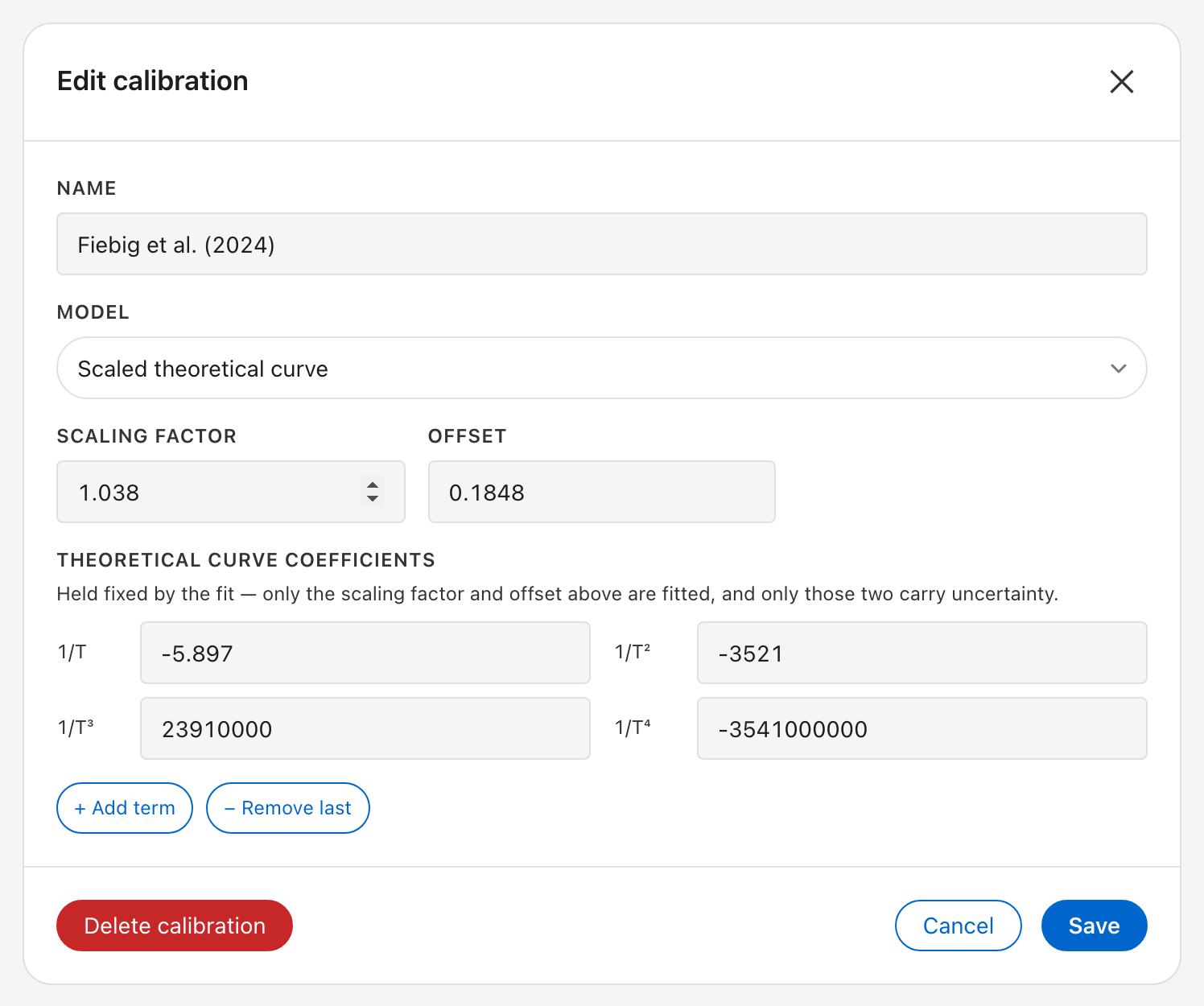
- Type the Scaling factor and the Offset. These are the two fitted numbers.
- Type the Theoretical curve coefficients, one per power of 1/T, as plain
numbers (for 2.391×10⁷, type
23910000or2.391e7). + Add term and − Remove last change the number of terms.
Delete calibration, in the Edit window, removes the equation.
Temperature conversion uses Δ₄₇ only.
δ¹⁸O Acid Fractionations
The minerals offered by the δ¹⁸O Acid Fractionation Correction card, each with
its reference and its a, b and c constants.
Chapter 5.1 explains how to turn a
published equation into these three numbers.
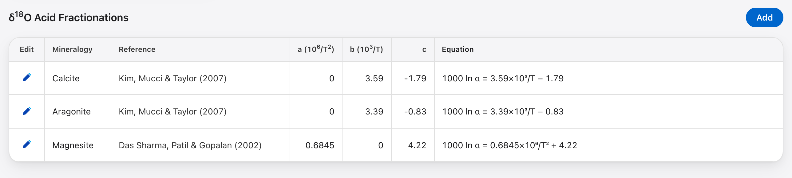
- Calcite, aragonite and magnesite are included.
- Add creates a new mineral; a pencil edits one. Type 0 for a term the paper's equation does not have.
- Delete mineral, in the Edit window, removes it. Samples that were assigned to it go back to "—" on the Standardization page.
- Every mineral needs a reference. One shown as Missing was carried over from an older version; edit it to add one.
- Calcite is also used by Bulk Standardization, to convert the standards' δ¹⁸O (chapter 5).
Display preferences
- Marker size: the size of the points in every plot, from 2 to 12.
- Default environment: which isotope system DELTALab starts on: Clumped Isotopes or Dual Clumped. Changing it does not switch the page you are on.
Additional Functions

Your databases. DELTALab works on one database at a time.
- New database creates an empty database. Choose where to save it, with Browse… or by pasting a full path, give it a Name and click Create. It never overwrites a file that already exists.
- Open database switches to another DELTALab database file. Choose it with Browse…, or paste its full path, and click Open. A file that is not a DELTALab database is refused.
- Rename database changes the name shown in the status bar and on its backups. The file on disk keeps its name.
After New database or Open database the app reloads on the chosen database, and DELTALab starts on it next time too.
Each database has its own sessions, Session History, attached files and reference material table. A new one starts with the shipped reference materials. The other settings on this page are shared by all your databases.
Backups.
- Back up now makes a backup at any moment.
- Restore backup opens the list of this database's backups.
- Export current saves a copy of the database you are using right now.
Chapter 8 explains when backups are made automatically, what an export contains and what a restore does.
Restore Default Settings resets the Reference material table, the computational variables and the temperature calibrations to the shipped values. Standards and calibrations you added or edited are lost.
- DELTALab asks you to confirm first and takes a safety backup, so you can undo it with Restore backup.
- It does not change mass spectrometers (or their reference gas and acid temperature), acid fractionation minerals, marker size, the default environment or your backups.
- It does not recalculate your sessions.
8. Backups, restore and updates
DELTALab keeps all your work in two files on your computer: the database
(sessions, raw acquisitions, results, Session History, attached files, reference
material table) and the settings file Storage.json (calibrations, minerals,
constants, instruments, display choices). A backup is a copy of both, taken together.
Where your data is
Both files start in the DELTALab data folder:
- macOS:
~/Library/Application Support/DELTALab/ - Windows:
%APPDATA%\DELTALab\
If you made or opened another database (chapter 7), it stays where you
put it. Hover over db: in the status bar to see its full path. Storage.json stays
in the data folder.
The backups are in a backups folder next to the database file, one folder per
backup. A backup's folder is named after its date and time, for example
20261005-154214, and holds database.zip and Storage.json.
Updating or reinstalling DELTALab does not touch the data folder.
Automatic backups
DELTALab makes a backup by itself:
- once a day, the first time you start the app that day. If an ordinary backup from today already exists, none is added;
- the first time you start a new version. This backup carries a label,
<old version> → <new version>, and is your way back if an update goes wrong; - the first time you open a database that day, with Open database;
- just before an action that removes or reshapes data:
- deleting a session;
- deleting replicates;
- renaming the sample of replicates;
- splitting a session;
- importing an Easotope database;
- Restore Default Settings;
- restoring a backup.
For each database, DELTALab keeps the newest 5 ordinary backups and, separately, the newest 3 labelled ones. A busy day of deletions can never push out an update backup, and the other way round.
Backups and restores are not written to Session History (chapter 4.3).
Making a backup or a copy
Both buttons are in Settings → Additional Functions (chapter 7).
- Back up now makes a backup at any moment, for example before a risky change. It is an ordinary backup: it is removed once five newer ones exist.
- Export current saves a copy of the database and settings you are using right now,
as a file named
DELTALab-database-<date and time>.zip. It holdsdatabase.dbandStorage.json.
Keep an export anywhere you like: an external drive, a shared folder, or send it to a colleague. An export is never removed by DELTALab, unlike backups. Export a copy whenever you want to keep a state for good.
Restoring a backup
- Go to Settings and click Restore backup. The window lists the backups of the open database, newest first, with their date and size.
- Click Restore on the backup you want.
- Confirm. DELTALab reloads.
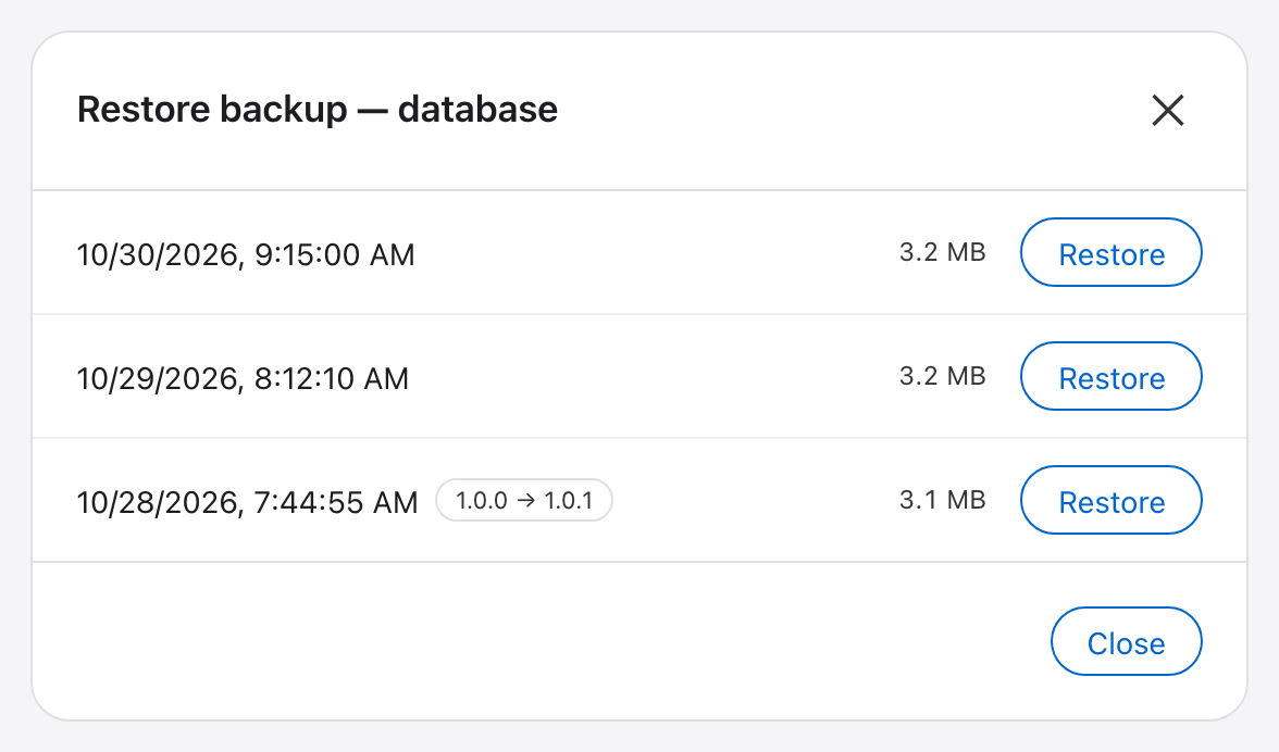
What the list can tell you:
- A label such as
1.0.0 → 1.0.1marks the backup taken before an update. - was "…" means the database had another name when the backup was made.
- database not recorded marks a backup too old to say which database it belongs to. Make sure it is the right one before you restore it; DELTALab asks you to check.
- A line at the bottom says how many backups of other databases in the same folder are not shown. Open that database to restore them.
What happens:
- The backup is checked first. A damaged backup is refused and nothing is changed.
- A safety backup of the current state is made, so a restore can always be undone. It appears at the top of the list.
- The database and the settings are replaced by the backup's. Everything you did after that backup is gone from the app: imports, processing, edits and changed settings. If you work with several databases, remember that the settings are shared by all of them.
To undo a restore, restore the safety backup that was made just before it.
Using an exported copy
Use this to bring an exported copy back, or to move your data to another computer.
- Quit DELTALab.
- Unzip the export.
- Put its
database.dbandStorage.jsonin the data folder, in place of the two files there. Keep the old ones somewhere else first if you may need them. - Start DELTALab.
Use a copy made with the same version of DELTALab, or an older one.
To look at an exported database without replacing anything, unzip it and use Open database. That keeps your current settings.
To look inside a backup without DELTALab: double-click its database.zip to
unzip it. The database.db inside is an SQLite database. Very old backups may
hold a plain database.db instead of a zip; both kinds restore correctly.
Updates
DELTALab checks for a new version each time it starts. When there is one, a banner appears under the top bar.

Marked in red: 1 the new version, 2 Update & Restart, 3 close the banner.
- Update & Restart (2) downloads the new version, installs it and restarts DELTALab. The banner shows "Downloading…" with a percentage while it works.
- × (3) closes the banner if you want to update later. It comes back the next time you start DELTALab.
- If your app is up to date, you see nothing.
- If the check or the installation fails, the banner says so and shows the error.
- On a computer DELTALab is not built for, the banner says that automatic updates are not available. Close it with ×.
Your data is not changed by an update. The first time the new version starts, it makes the labelled backup described above.
If an update goes wrong, go back to the version you had:
- Restore the backup labelled with the version you came from (Settings → Restore backup).
- Quit DELTALab.
- Install that older version again. It is the one on the left of the arrow in the label.
Your data is then exactly as it was before the update. Anything you did in the new version is not in it; it is in the safety backup the restore made.
DELTALab is built for Macs with Apple Silicon and for 64-bit Windows. Only some versions are also built for Intel Macs, and none for Windows on ARM. When the newest version was not built for your computer, there is nothing to update to and DELTALab says so.
Developer documentation: see ARCHITECTURE.md and .claude/rules/ in the source
code.